Case Study 4: Summarizing Model Outputs
Introduction and Learning Objectives
This case study is designed to get you familiar with constructing and summarizing a Markov model in Excel. Specific learning objectives are as follows:
Parameterize and structure a Markov model.
Embed a transition probability matrix using rate-to-probability conversion formulas
Summarize average total costs and QALYs using cycle adjustments and discounting.
Calculate incremental cost-effectiveness ratios.
Overview of Decision Problem
As in earlier case studies, we will examine a preventive health measure designed to protect against the onset of a disease (“sick”):
- All patients start out healthy (utility weight = 1.0)
- Becoming sick reduces utility to 0.75 and carries yearly treatment costs $1000 .
- Becoming sick substantially increases the likelihood of death (Hazard Ratio =3).
- Population cohort starts at age 25 and is followed until age 100 (or everyone dies).
- Background mortality is based on life table data.
Treatment Options
The standard of care (Treatment “A”) is a preventive measure (e.g., a drug, screening program, etc.) that costs $25 per yr. However, there are several new preventive measures with varying costs and effects:
| Strategy | Cost | Hazard Ratio of Becoming Sick (Reference for HR: Strategy A) |
|---|---|---|
| A | 25 | |
| B | 1000 | 0.96 |
| C | 3100 | 0.88 |
| D | 1550 | 0.92 |
| E | 5000 | 0.92 |
Our primary decision problem, then, is to determine whether the Ministry of Health should adopt a new preventive measure.
Part 1. Parameterize the Model
As before, our first step is to define variable names for all the inputs parameters in our decision problem. Again, the blog posting on useful Excel functions covers how to assign variable names in detail, and using several methods.
Use variable names to assign values to each parameter in the Excel document. NOTE: This is already completed in the workbook, but feel free to complete it yourself again!!
You may notice that the orange-shaded variables at the bottom do not change once we define variables for all its inputs. To fix this, in the base_case column, simply add an “=” sign to the formulas, as you did in the last case study. After doing so, the numeric value for these variables should appear.

You will also notice that in each treatment strategy worksheet there is a “Payoffs” table. This table has a corresponding cost and utility for each health state—and these payoffs will differ by strategy due the different costs of each.

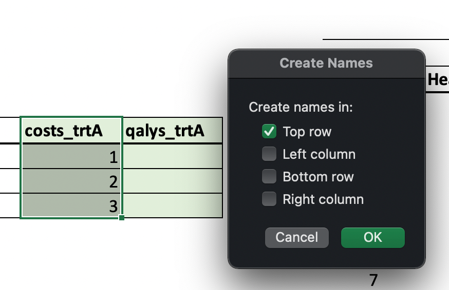
Using the variable names you defined in the parameter worksheet, fill out the payoff tables in each strategy worksheet. Make sure to assign each column to the name at the top (e.g., costs_trtA is the vector of costs for Healthy, Sick and Dead; see margin note)
You can define a name for a vector of payoffs much like you defined a name for the transition probability matrix:
Part 2: Calculating Costs, QALYs, and Cycle Adjustments for Each Time Period
Markov Trace
We will again construct a Markov trace for each of strategies.
Construct a Markov trace for each strategy. Note this exercise is a repeat of the exercise in Case Study 3. NOTE: This is already completed in the workbook, but feel free to complete it yourself again!!
Total Costs and QALYs in Each Cycle
Once our Markov traces are complete, our next step is to calculate the total costs and QALYs in each cycle. For example, for cycle 1 suppose 95% of the population is healthy, 4% is sick and 1% have died. Suppose that there is no cost to being healthy or dead, and being sick carries a $5,000 cost. In cycle 1, the total average costs costs are $200 = 0 * 0.95 + 5000 * 0.04 + 0 * 0.01.
Similarly, we can calculate total QALYs for a cycle by multiplying state occupancy (i.e., the fraction of the population in a given category) by the utility (rather than cost) weight for each health state.
There are two equivalent ways to calculate total costs/QALYs for each cycle. First, you could simply do the math “by hand” by multiplying state occupancy by the cost/utility value in the payoff table; this is the approach used above to calculate an average total cost of $200 in the first cycle.
Alternatively, you can construct the total cost/QALY column all at once by doing matrix multiplication of the Markov trace and the payoff vector, i.e., MMULT(TRACE,PAYOFF). See the video in the margin for an example of both methods.
Use the cost and QALY payoff vectors you defined in Exercise 4.2, along with the Markov trace you defined in 4.3, to calculate total cycle costs and utilities for strategies A through E. Make sure to assign each column to the variable name at the top!
You can calculate total costs “by hand” by simply multiplying each payoff by the fraction of the population in that state, and then adding together. Or, you can use matrix multiplication to do it in one step. To do this, multiply the entire Markov trace by the payoff vector: MMULT(TRACE, PAYOFF). See the video below for an example of both methods.
Discounting and Cycle Adjustments
Before we can calculate average total costs and QALYs across all cycles, we need to ensure that we discount and implement a cycle adjustment, as was covered in the lecture. To do this, for each outcome (costs, QALYs) we will construct three new columns in each worksheet:
- A column with the discount value for each cycle.
- A column with the cycle adjustment value for each cycle.
- A column that multiplies #1 and #2 – this is our total cycle adjustment value.
Discounting
As covered in the lecture, we calculate the the discount value for a given cycle \(t\) as
\[ 1 / (1 + d_r)^{t} \]
where \(d_r\) is the discount rate (e.g., 0.03) and \(t\) is the cycle number. The table below provides cycle discount values for three cycles in a model, based on a discount rate (\(d_r\)) of 0.3:
| cycle | formula | value |
|---|---|---|
| 0 | 1/(1+0.03)^0 | 1 |
| 1 | 1/(1+0.03)^1 | 0.97087 |
| 2 | 1/(1+0.03)^2 | 0.9426 |
| … | … | … |
Note that in the parameters table we define two discount rates: one for costs (i.e., d_c) and one for utility (i.e., d_e). Often these values will be the same (e.g., 3%), however we define them seprately to give us the the flexibility to assign different discount rates for costs and QALYs in our model.
Fill in the discount rate value for each cycle in each strategy worksheet. Note that you will need to do this separately for costs (using d_c) and QALYs (using d_e).
Cycle Adjustment
For this exercise we will use Simpson’s 1/3 rule to implement a cycle adjustment–though in principle, a half-cycle correction, the trapezoidal rule (i.e., life-table method), or some other numerical integration method could be used.
Implementing Simpson’s rule is straightforward. The cycle adjustment values are based on the following process:
- Enter a value of 1/3 in first and last cycle
- Alternate values of 4/3 and 2/3 in between.
Fill in cycle adjustment value for each cycle in each strategy worksheet.

Total Cycle Adjustment
We now have the ingredients we need to calculate a total cycle adjustment value.
Calculate the total cycle adjustment value (i.e., discounting multiplied by the cycle adjustment). Don’t forget to name this vector using the name supplied at the top of the column!
Part 3: Average Total Costs and QALYs
We are now prepared to calculate the total (discounted) costs and QALYs for each strategy. Again, we can do this by hand or in one step using matrix multiplication.
To manually calculate total average costs and QALYs, we go cycle by cycle and multiply the total costs/QALYs (calculated in the section titled “Total Costs and QALYs in Each Cycle”) by the corresponding total cycle adjustment value (calculated in the section titled “Total Cycle Adjustment”). We then sum up these values across all cycles to cacluate the final average total cost/QALY value.
An alternative (faster) way to do this is again using matrix multiplication:
MMULT(TRANSPOSE(cost_adjustment),total costs)MMULT(TRANSPOSE(qaly_adjustment),total QALYs)
In the excel functions above, TRANSPOSE() simply flips the cost/QALY adjustment column from a long column to a long row; we must do this to ensure the matrix multiplication works correctly.
The matrix multiplication process outlined above will produce a single total average cost/QALY value; it is equivalent to the value you would get after summing across cycles in the first (“by hand”) approach.
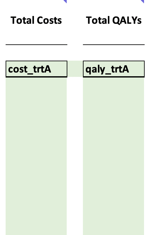
In your Excel document, you’ll see a small table on the far right in each strategy worksheet:

Calculate the total average costs and QALYs for each strategy Don’t forget to name these values using the name supplied at the left of the table!
Identifying Dominated Strategies and Calculating Incremental Cost-Effectiveness Ratios
Once you have calcuated total average costs and QALYs for each strategy, you are ready to move to the final worksheet titled ICER. In this worksheet, we will determine dominated strategies and will construct a final table summarizing our base case decision model results.
Enter Total Costs and QALYs for each strategy
The top table in the ICER worksheet has columns for Strategy, Cost and Effect
Enter the total cost and QALY estimates for each strategy name into these columns.
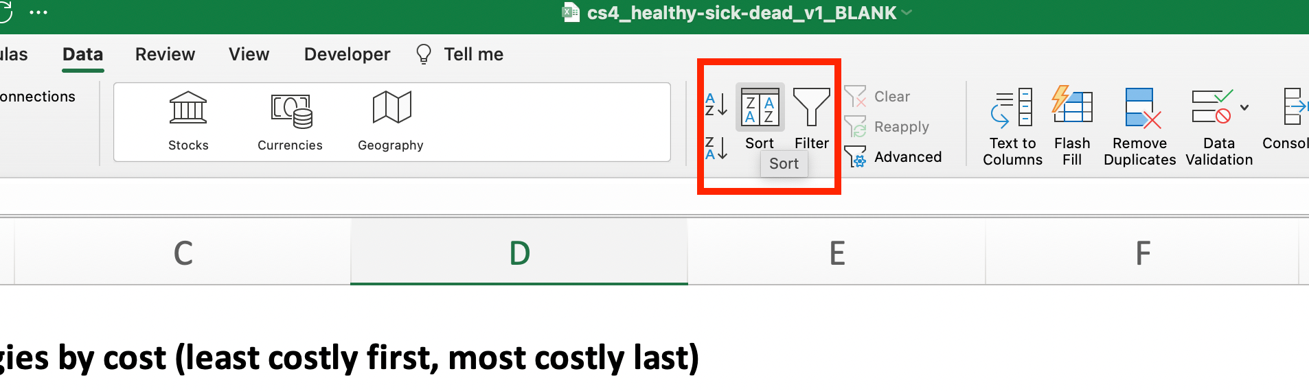
An important next step is to sort this table by ascending costs. You can do this by selecting the range of cells you wish to sort, then clicking on the “Data” ribbon and clicking the “Sort” button:
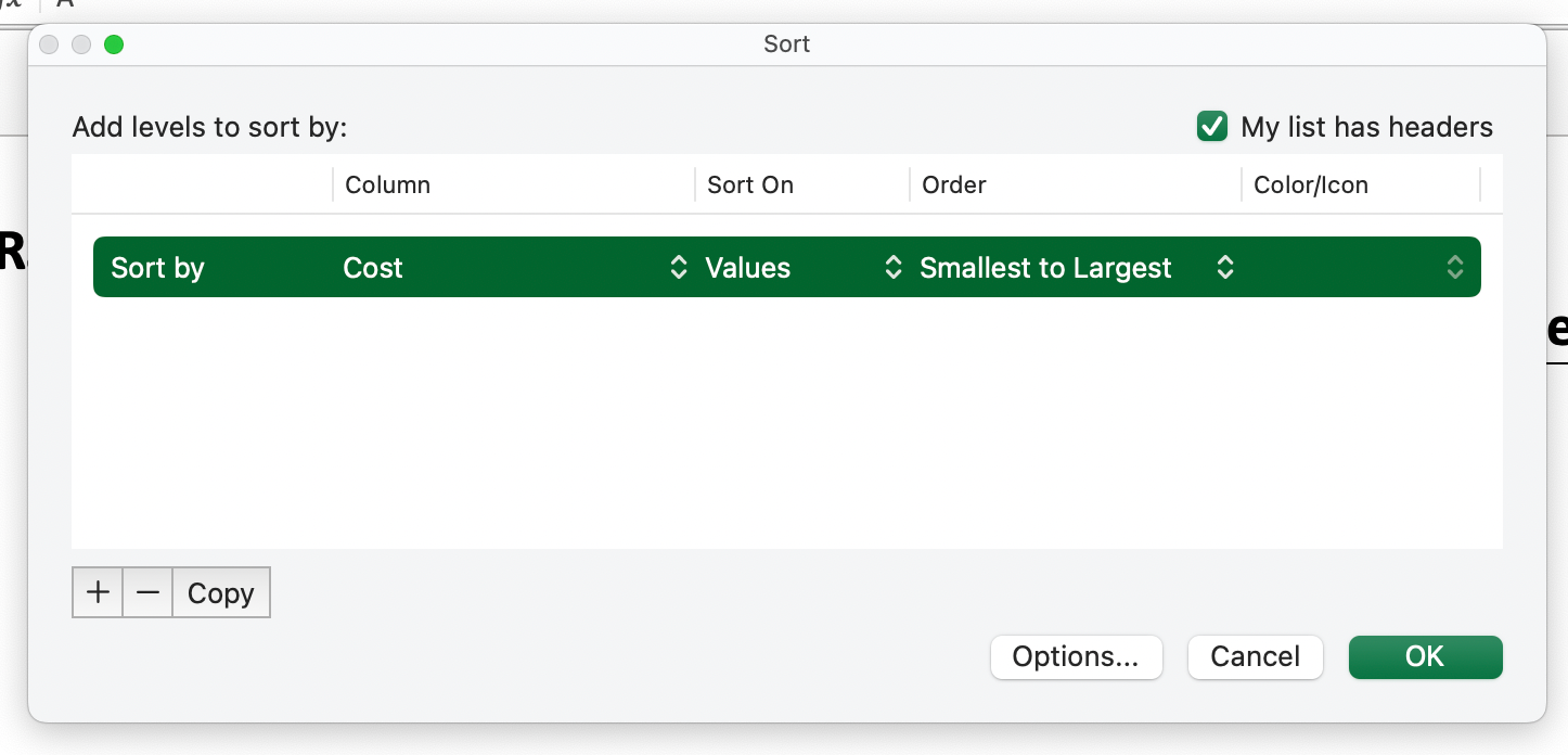
The popup box that appears will allow you to sort by “Column,” where you can select the “Cost” column, and ensure that it is sorting by “Smallest to Largest”.
Calculate the Initial ICERs for Each Strategy
Once you have done this, you are ready to construct the first set of ICERs.
Fill in the incremental cost and incremental effect columns, and use the values in these columns to calclate the incremental cost-effectiveness ratio (ICER column).
Remove strategies that are strictly dominated
Once you have ICERs, take a look at them. Are any of them strictly dominated? That is, are there any strategies that are less effective than their comparator, but cost more?
Identify any dominated strategies and note that they are dominated in the “Status” column in the table titled Initial ICERs.
Next, we will construct a new ICER table after we take any dominated strategies out of consideration. To do this, simply copy and paste the Strategy, Cost and Effect columns from your initial table into the second table on the worksheet.
Once you have filled out the Strategy, Cost and Effect columns in the table titled “Remaining strategies when strictly dominated strategies are removed,” recalculate the ICERs using the same process as above.
Remove strategies subject to extended (weak) dominance
Our next step is to identify and remove weakly dominated strategies from consideration. These are strategies that have an ICER that is higher than the next most expensive strategy in the table.
Identify any weakly dominated strategies and note that they are weakly dominated in the “Status” column in the table.
We can now remove the weakly dominated strategies from consideration and move to the next table in the worksheet.
Construct the Final ICER Table
Once we have identified and removed all weakly dominated strategies, we’ll construct a new table with ICERs for all remaining strategies.
Construct the table titled “Final ICERs after all weakly dominated strategies are removed”. To do this you should use the same process as above.
Construct a Final Table for Reporting
With the ICERs all calculated, its now time to summarize our findings across all strategies. That is, we don’t want to only report strategies with a defined ICER; we also want to report on the status of dominated strategies as well.
Construct the final table. This table should include all strategies and their ICER, or their (dominated) status.