7. Summarizing model outputs

Learning Objectives and Outline

Learning Objectives

Be able to derive summary outcomes (costs and health outcomes) from a Markov trace
Be able to apply methods for:
- Cycle correction
- Discounting a stream of costs (or benefits) and calculating net present value
- Adjusting costs measured in different currencies to a common currency (and currency year)

Outline

Calculating Life Years
Cycle correction
Inflation Adjustment
Currency Conversion
Discounting
Calculating Total Costs and QALYs

Calculating Life Years

A Markov trace from Case Study 2…

Cycle	Healthy	Sick	Dead
0	1.000	0.000	0.000
1	0.856	0.138	0.007
2	0.732	0.253	0.015
3	0.626	0.349	0.025
4	0.536	0.429	0.035
5	0.458	0.495	0.046
…	…	…	…
75 (End)	0	0.282	0.718

Life years

Life years = cumulative “reward” of being in an “alive” (healthy or sick) state

Cycle	Healthy	Sick	Dead	LY (single cycle)
0	1.000	0.000	0.000	1
1	0.856	0.138	0.007	0.856 + 0.138 = 0.993
2	0.732	0.253	0.015	0.732 + 0.253 = 0.985
3	0.626	0.349	0.025	0.975
4	0.536	0.429	0.035	0.965
5	0.458	0.495	0.046	0.954
…	…	…	…
75 (End)	0	0.282	0.718	0.282

Life years

Cycle	Healthy	Sick	Dead	LY (single cycle)	LY (cumulative)
0	1.000	0.000	0.000	1	1
1	0.856	0.138	0.007	0.993	1 + 0.993 = 1.993
2	0.732	0.253	0.015	0.985
3	0.626	0.349	0.025	0.975
4	0.536	0.429	0.035	0.965
5	0.458	0.495	0.046	0.954
…	…	…	…	…
75 (End)	0	0.282	0.718	0.282

Life years

Cycle	Healthy	Sick	Dead	LY (single cycle)	LY (cumulative)
0	1.000	0.000	0.000	1	1
1	0.856	0.138	0.007	0.993	1.993
2	0.732	0.253	0.015	0.985	1 + 0.993 + 0.985 = 2.978
3	0.626	0.349	0.025	0.975
4	0.536	0.429	0.035	0.965
5	0.458	0.495	0.046	0.954
…	…	…	…	…
75 (End)	0	0.282	0.718	0.282

Life years

Cycle	Healthy	Sick	Dead	LY (single cycle)	LY (cumulative)
0	1.000	0.000	0.000	1	1
1	0.856	0.138	0.007	0.993	1.993
2	0.732	0.253	0.015	0.985	2.978
3	0.626	0.349	0.025	0.975	3.954
4	0.536	0.429	0.035	0.965	4.919
5	0.458	0.495	0.046	0.954	5.872
…	…	…	…	…	…
75 (End)	0	0.282	0.718	0.282	44.825

The cumulative LYs for an individual starting in the Healthy state is 44.825
Note that this is within a 75 years time horizon
- They may still be alive and keep accumulating LYs if we extend the time horizon

Cycle correction

The problem

Time is continuous, so are survival/event-free survival curves
When we discretize time by using a fixed cycle length, we can make two assumptions
- Suppose this is a simple Well $\rightarrow$ Dead process

The problem

Assuming death happens at the end of cycle (A)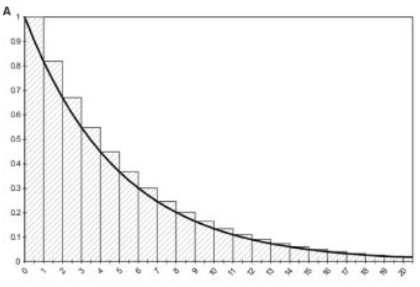

Overestimates state membership in Well

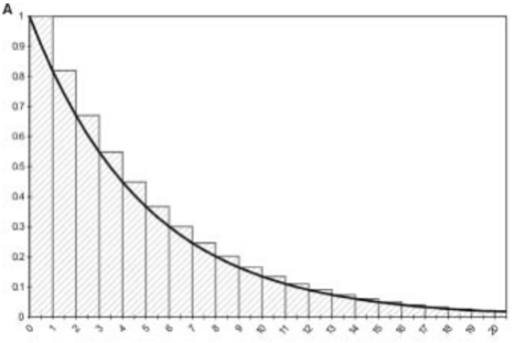
Assuming death happens at the start of cycle (B)

Underestimates state membership in Well

Source

Methods to address this problem

Half-cycle correction
Simpson’s 1/3 correction

Half-cycle correction

Source

Half-cycle correction

Source

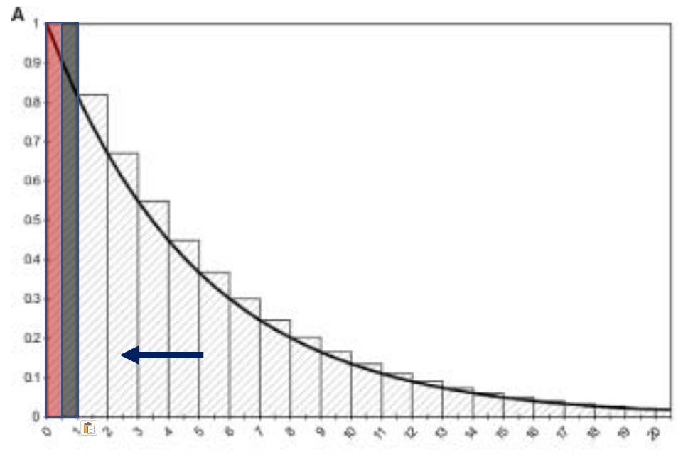
Half-cycle correction

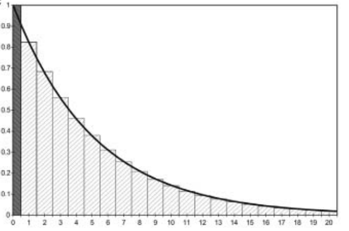
Multiply the outcomes by 1/2 in the first and last cycle.
Shifting the computed, discrete state membership curve to the left by 1/2 cycle.
Essentially assuming that events happen in the middle of cycle

Source

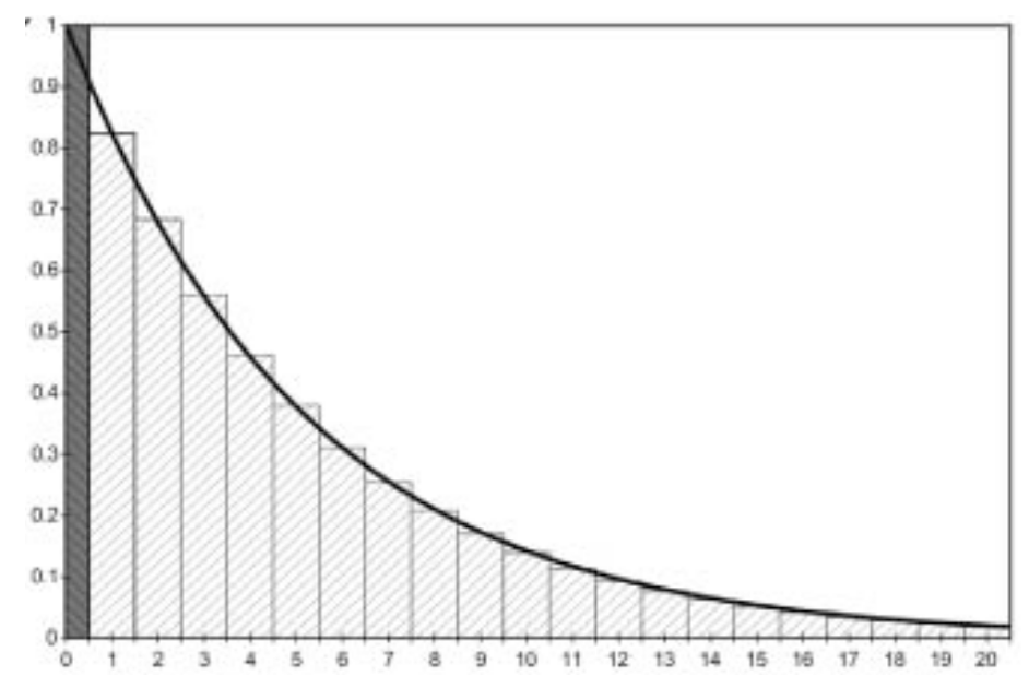
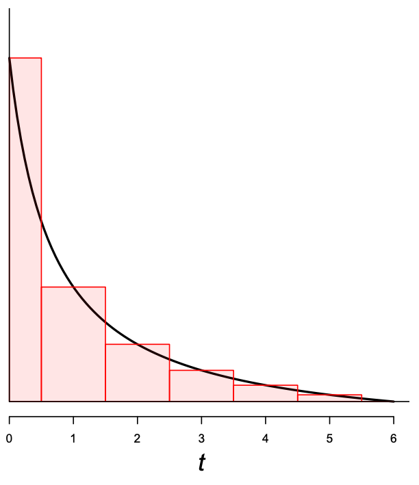
Half-cycle correction

It can still be imprecise, especially when there’s more curvature in the true, continuous curve:

Source

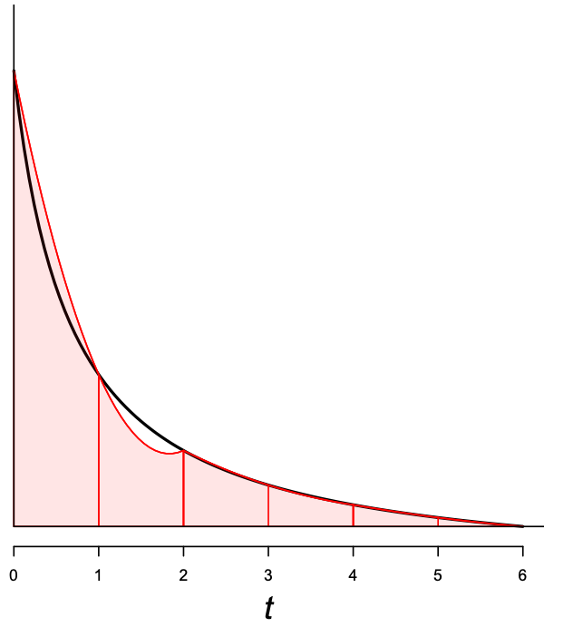
Simpson’s 1/3 Correction

Uses the area under the quadratic curve passing through 3 points {$t_{k-1}, t_{k}, t_{k+1}$}
Multiply the outcomes by 1/3 in the first and last cycle.
Multiply the outcomes by 4/3 if the cycle number is odd and by 2/3 if the cycle number is even.
Note that the time horizon must be even $\leftarrow$ This formation requires 2 sub-intervals from $t_{k-1}$ to $t_{k+1}$

Source

Comparison of Methods: Summary

Standard half-cycle correction is the most widely used approach
Simpson’s 1/3 method performs the best among existing methods (It converges to the continuous-time exact solutions the fastest)
The choice of method matters less with shorter cycle length
To learn more: Elbasha EH, Chhatwal J. Theoretical Foundations and Practical Applications of Within-Cycle Correction Methods. Med Decis Making. 2016 Jan 1;36(1):115–31.

Apply cycle correction methods to our CS2 markov trace…

Half-cycle correction

Multiply the outcomes by 1/2 in the first and last cycle.

Cycle	Healthy	Sick	Dead	LY (single cycle, adjusted)	LY (cumulative)
0	1.000	0.000	0.000	1*0.5	0.5
1	0.856	0.138	0.007	0.993	0.5 + 0.993 = 1.493
2	0.732	0.253	0.015	0.985	2.478
3	0.626	0.349	0.025	0.975	3.454
4	0.536	0.429	0.035	0.965	4.419
5	0.458	0.495	0.046	0.954	5.372
…	…	…	…	…	…
75 (End)	0	0.282	0.718	0.282 *0.5	44.184

This number is smaller than our original estimate without half-cycle correction (44.825!)

Simpson’s 1/3

Multiply the outcomes by 1/3 in the first and last cycle.
Multiply the outcomes by 4/3 if the cycle number is odd and by 2/3 if the cycle number is even.
Note that the time horizon must be even.

Cycle	Healthy	Sick	Dead	LY (single cycle	Cycle Adjustment	LY (single-cycle, adjusted)	LY (cumulative)
0	1.000	0.000	0.000	1	0.333	1*0.333 = 0.333	0.333
1	0.856	0.138	0.007	0.993	1.333	0.993*1.333 = 1.324	1.657
2	0.732	0.253	0.015	0.985	0.667	0.985*0.667 = 0.657	2.314
3	0.626	0.349	0.025	0.975	1.333	…	…
4	0.536	0.429	0.035	0.965	0.667	…	…
5	0.458	0.495	0.046	0.954	1.333	…	…
…	…	…	…	…	…	…	…
75	0	0.282	0.718	0.282	1.333	0.282*1.333 = 0.376	…
76 (End)	0	0.277	0.723	0.277	0.333	0.277*0.333 = 0.092	44.454

Introducing some other adjustments before we get to calculating costs and QALYs…

Inflation adjustment (cost)
Currency conversion (cost)
Discounting (both cost and health)

Inflation Adjustment

Inflation Adjustment: Motivation

$100 in 2000 is not equivalent to $100 in 2020
- $100 could buy a lot more in 2000!
Important to adjust for the price difference over time, especially when working with cost sources from multiple years

Inflation Adjustment: Method

Choose a reference year (usually the current year of analysis)
Convert all costs to the reference year

Converting cost in Year X to Year Y (reference year):

\[ \textbf{Cost(Year Y)} = \textbf{Cost(Year X)} \times \frac{\textbf{Price index(Year Y)}}{\textbf{Price index(Year X)}} \]

Inflation Adjustment: Example

Cost of hospitalization for mild stroke in the US was ~15,000 USD in 2013. What if we want to convert this number to 2020 USD?

CPI (Consumer Price Index) in 2013: 233
CPI in 2020: 259 (Source: US Bureau of Labor Statistics)

\[ \textbf{Cost(2020)} = \textbf{Cost(2013)} \times \frac{\textbf{CPI(2020)}}{\textbf{CPI(2013)}} \\ = 15,000 \times \frac{259}{233} \\ = 16,674 \ (\text{2020 USD}) \]

Currency Conversion

Isn’t required for CEA but may be useful in some situations:
- Example: may need to convert local currency to USD because cost-effectiveness thresholds are often estimated in the unit of USD per DALY.
Taking the capstone Rotavirus example, how do we convert 100 Indian Rupees to USD?
Current exchange rate in 2022: 1 Indian Rupee = ~0.12 USD
100 Indian Rupees = 12 USD

Discounting

Why discounting?

Adjust costs at social discount rate to reflect social “rate of time preference”
- Pure time preference (“inpatience”)
- Potential catastrophic risk in the future
- Economic growth

How do we discount?

Present value: $PV = FV/(1+r)^t$
- FV = future value, the nominal cost incurred in the future
- r = annual discount rate (analogous to interest rate)
- t = number of years in future when cost is incurred
Reasonable consensus around 3% per year
May vary according to country guidelines

Adjust for inflation and currency first, then discount

Intuition

$r = 0.03$
Recall that $PV = FV/(1+r)^t$, and we’re at Year 0:
- $1 in Year 0 is valued as $1/1.03^0 = \$ 1$
- $1 in Year 1 is valued as $1/1.03^1 = \$0.97$
- $1 in Year 2 is valued as $1/1.03^2 = \$0.94$
- $1 in Year 3 is valued as $1/1.03^3 = \$0.92$
- …

Example

Assume in year 5, a patient develops disease, and there is a treatment cost of $500
- This is the future value (FV) of the cost!
Present value PV = $PV = FV/(1+r)^t = 500/(1+0.03)^5 = \$ 431.3$

Discounting health benefits

The consensus is that health benefits should be discounted at the same rate as costs
- May vary in some country guidelines
Why?

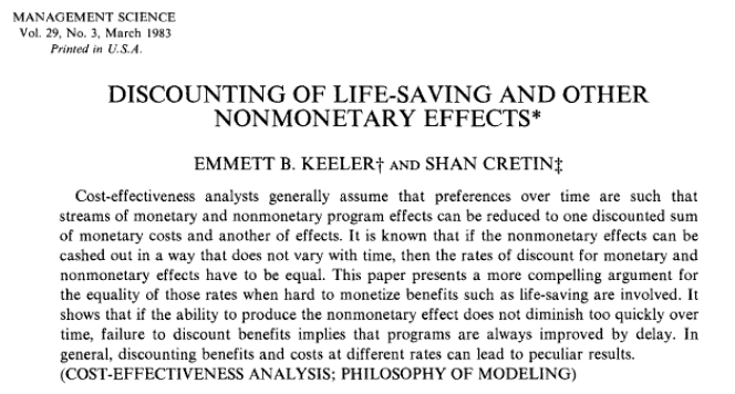
The Keeler-Cretin Paradox

Imagine that an intervention would cost $100,000 and yield a 1 QALY benefit. If we discount costs at 3% per year but don’t discount QALYs…

If implementing this intervention in year 0…

	Year 0
Cost ($)	100,000
Health Benefit (QALY)	1
ICER ($/QALY)	100,000

The Keeler-Cretin Paradox

Imagine that an intervention would cost $100,000 and yield a 1 QALY benefit. If we discount costs at 3% per year but don’t discount QALYs…

If implementing this intervention in year 1…

	Year 0	Year 1
Cost ($)	100,000	100,000/1.03 = 97,087
Health Benefit (QALY)	1	1
ICER ($/QALY)	100,000	97,087

The Keeler-Cretin Paradox

Imagine that an intervention would cost $100,000 and yield a 1 QALY benefit. If we discount costs at 3% per year but don’t discount QALYs…

If implementing this intervention in year 2…

	Year 0	Year 1	Year 2
Cost ($)	100,000	100,000/1.03 = 97,087	100,000/(1.03^2) = 94,260
Health Benefit (QALY)	1	1	1
ICER ($/QALY)	100,000	97,087	94,260

This is where the paradox arises: It seems more favorable to indefinitely delay the intervention!

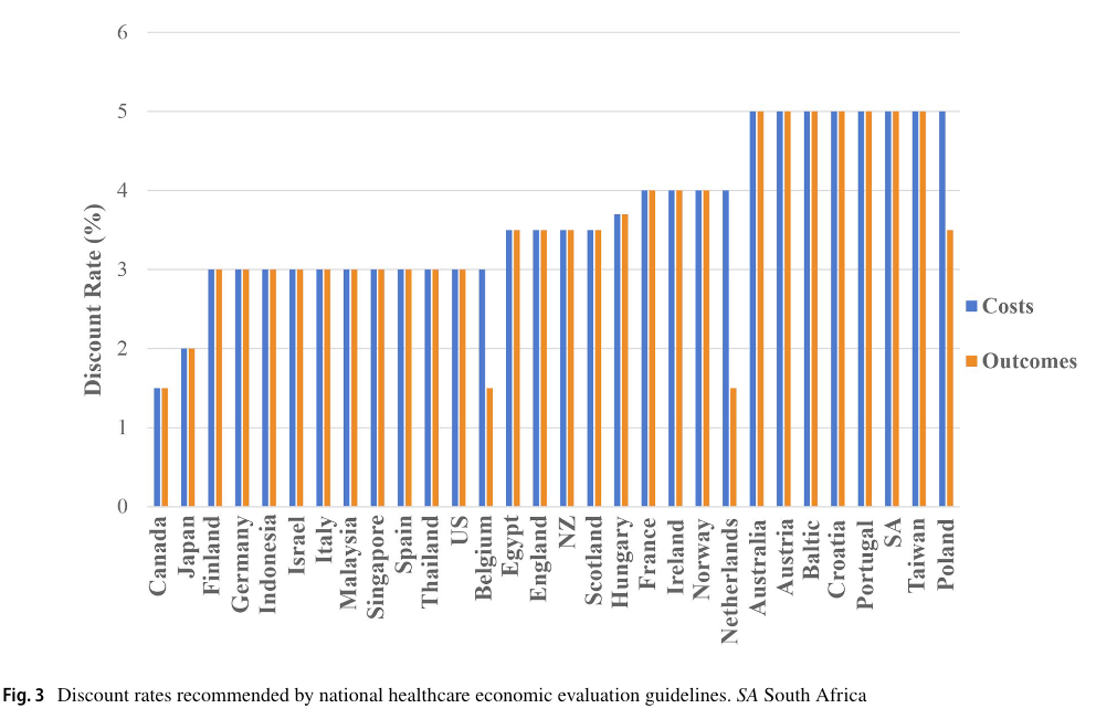
Discounting rates – Cross-country comparison

Source

Calculating Costs and QALYs

Costs and QALYs can be accumulated similarly as “rewards” separately
Costs:
- (Transform all costs into the same currency and currency year before entering them into the model)
- Cycle correction
- Discounting
QALYs:
- Utility weight
- Cycle correction
- Discounting

Calculating Costs and QALYs

We will practice how to perform all adjustments simultaneously to calculate total costs and QALYs from a Markov trace in Case Study 4!