Case Study 5: Deterministic Sensitivity Analysis
Introduction and Learning Objectives
This case study is designed to get you familiar with conducting deterministic sensitivity analysis in Excel. Specific learning objectives are as follows:
- Explain the purpose of deterministic sensitivity analysis and provide examples of one-way versus two-way analyses.
- Detail the advantages/disadvantages of deterministic sensitivity analysis.
Overview of Decision Problem
As in earlier case studies, we will examine a preventive health measure designed to protect against the onset of a disease (“sick”):
- All patients start out healthy (utility weight = 1.0)
- Becoming sick reduces utility to 0.75 and carries yearly treatment costs $1000 .
- Becoming sick substantially increases the likelihood of death (Hazard Ratio =3).
- Population cohort starts at age 25 and is followed until age 100 (or everyone dies).
- Background mortality is based on life table data.
Treatment Options
The standard of care (Treatment “A”) is a preventive measure (e.g., a drug, screening program, etc.) that costs $25 per yr. However, there are several new preventive measures with varying costs and effects:
| Strategy | Cost | Hazard Ratio of Becoming Sick (Reference for HR: Strategy A) |
|---|---|---|
| A | 25 | |
| B | 1000 | 0.96 |
| C | 3100 | 0.88 |
| D | 1550 | 0.92 |
| E | 5000 | 0.92 |
Our primary decision problem, then, is to determine whether the Ministry of Health should adopt a new preventive measure.
Base Case Summary
In Case Study 4, we calculated total average costs and QALYs, as well as ICERs, when all model parameters were set at their baseline (i.e., “base case values”):
| Strategy | Costs ($) | QALYs | Incremental Costs ($) | Incremental QALYs | ICER ($/QALY) | Status |
|---|---|---|---|---|---|---|
| A | 16,454 | 17.33 | ||||
| D | 24,504 | 17.49 | 8,050 | 0.16 | 50,478 | |
| C | 33,443 | 17.58 | 8,939 | 0.09 | 101,292 | |
| B | 21,457 | 17.41 | ED | |||
| E | 43,332 | 17.49 | D | |||
| ED = Dominated (Extended) D=Dominated | ||||||
Figure 1 makes clear that with a willingness-to-pay (i.e., \(\lambda\)) threshold of $50,000 / QALY we would select strategy A—however the ICER for Strategy D is quite close to our threshold. How sensitive is this decision to the specific values of the parameters used?
Setting Low and High Values for Determininistic Sensitivity Analysis
As covered in the lecture slides, there are two primary methods for evaluating the effects of uncertainty on model results and decisions: deterministic (one-way) sensitivity anslysis and probabilistic sensitivity analyses (PSAs).
In a deterministic sensitivity analysis, we allow uncertain parameters to vary one at a time while holding all other model parameters fixed at their base case values.
Conducting a “What-If” Analysis In Excel
Deterministic sensitivity analyses can be done in Excel using the built in “What-If Analysis” features. These can be found in the “Data” ribbon:

To see how the “What If” feature works, let’s define a very simple “model” with a single input parameter (input_param) and four outcomes:
- Outcome 1:
input_param+10 - Outcome 2:
input_param$*$10 - Outcome 3:
input_param/100
In Excel we construct the model in a single worksheet in which we define the parameter input_param with an initial value of 10, and calculate all three outcomes:

You can think of these initial outcome values like the outcomes from a “base case” model run. A sensitivity analysis could then ask: what would outcomes look like under different values for input_param?
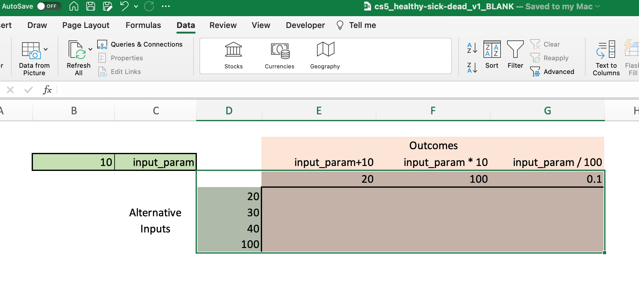
To explore outcomes under different input values, we can expand the table in Figure 2 to include alternative values for input_param:

Note that we now have two “flavors” of inputs:
- The primary (“base case”) model input for
input_paramof 10, which is contained in cell B3. - Alternative values for
input_param, which are contained in the range D5:D8.
We will next fill in the “What If” analysis table using the Data Table function in Excel.
First, select only the cells with the input and output values you want in the Data Table. This selection is shown in the figure below:
Clicking on the “What-If Analysis” button in the Data panel gives us the following:
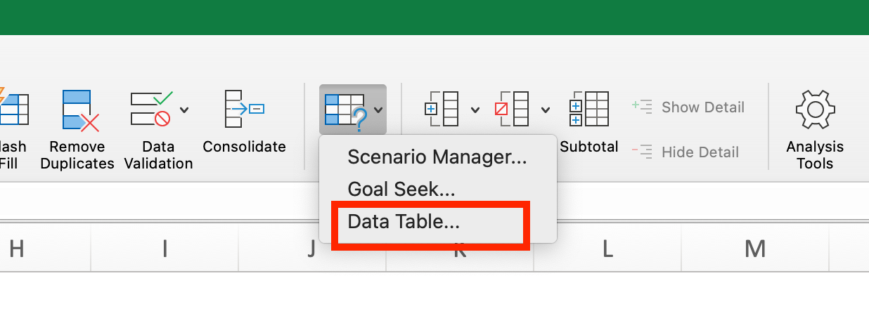
You should select “Data Table” in the popup box. Once you do, a popup diaglog box will appear with an option for the “Row input cell” and an option for the “Column input cell.” Which should we use?
In this example, our primary input (input_param) is contained in cell B3 and our primary outputs are contained in columns E through G. Therefore, our Column input cell is cell B3 in the spreadsheet.
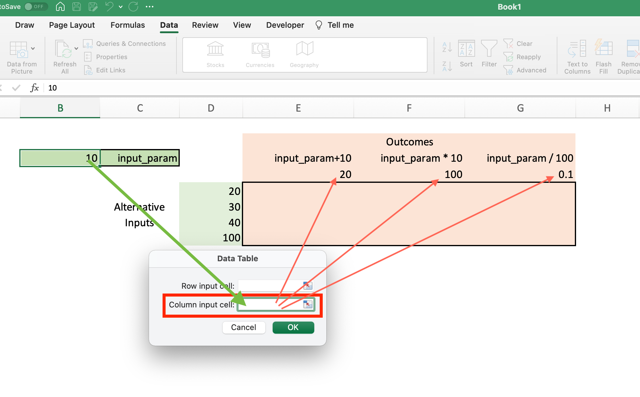
Once you enter B3 into the Column input cell area, you can click “OK” and the rest of the table will fill out. What happens when it does?
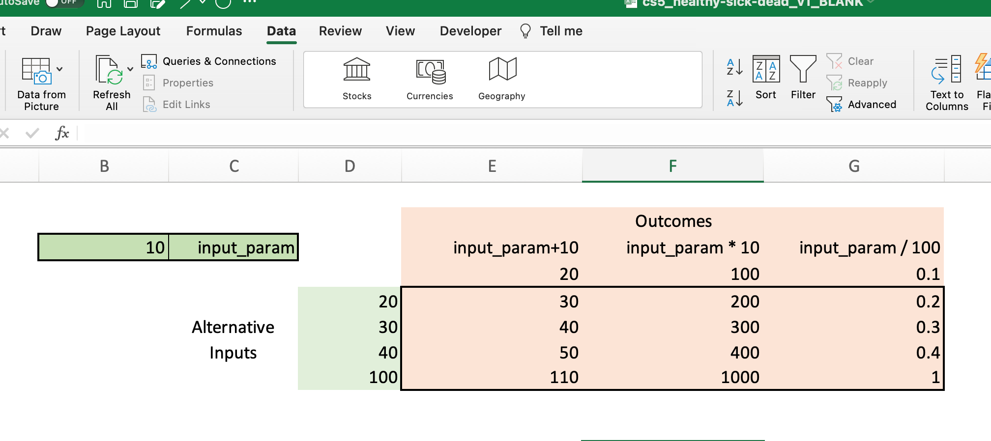
Essentially, Excel will take each of the alternative input values (i.e., those in column D) and run them as the value of the input_param variable in the model. The outcome from this model run will then be shown under each column in the table.
For example, first Excel will use a value of 20 for input_param. The “model” will then return a outcome values of 30 (20+10), 200 (20*10) and 0.2 (20/100). The next row will show the outcome values when input_param is set to 30, 40, etc.
The full data table is shown below:
Using Row Input Values
An equally valid alternative way to do the above is to structure the Data Table such that the inputs are in the columns and the outputs in the rows of the table. In that case, you would enter B3 as the Row input cell rather than the column input cell, as shown below:
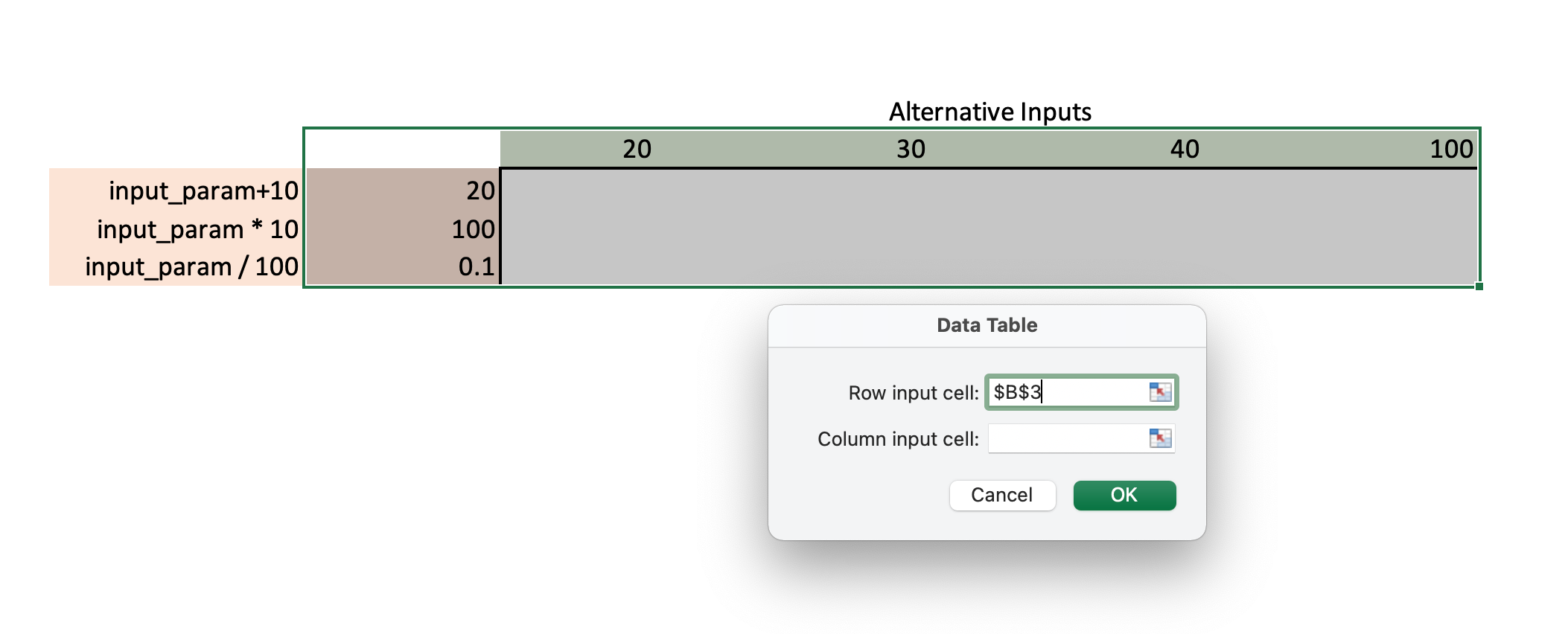
Once you hit “OK” the table will automatically calculate:

Note that we will use this “Row input cell” approach for the sensitivity analysis exercise in the Healthy-Sick-Dead model below.
Deterministic Sensitivity Analysis for the Healthy-Sick-Dead Model
We can conduct a deterministic (one-way) sensitivity analysis on our healthy-sick-dead model using the Data Table feature, as we did above.
A key limitation of Excel is that the “Column input cell” must be on the same worksheet as the Data Table you are constructing. Therefore, your deterministic sensitivity analysis for this exercise should be done in the parameters worksheet in the Excel document.
Step 1: Define the Variables for the Deterministic Sensitivity Analysis
Our first step is to identify the parameters we wish to vary in the sensitivity analysis. For each of these uncertain parameters, we want to explore model outcome sensitivity to different values of the parmeters while holding all other model parameters fixed at their base case values.
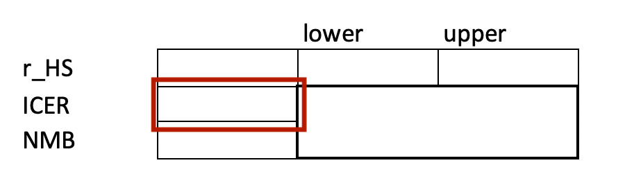
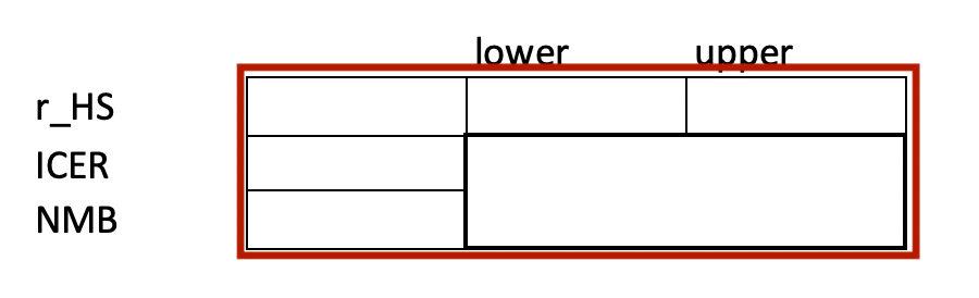
In the case study Excel document, navigate to the parameters worksheet. Ohe far right you will notice that a table shell for a single input parameter (r_HS) has already been created for you.

Create Data Table shells for 5-6 uncertain parameters in your model. These should be done in the same columns (L through O) as in the Excel file.
For now, don’t worry about the lower and upper values; just create empty table shells as was done for r_HS.
Step 2: Define the Lower and Upper Values for the Sensitivity Analysis
With our Data Table shells created, we will next turn to defining the upper and lower values we wish to consider.
Best practice recommends defining these values based on published evidence (e.g., the upper and lower values of the 95% confidence interval for the parameter, if it is based on a published value).
Alternatively, we could define an uncertainty distribution for each parameter and assign values at the 2.5th and 97.5th percentile (or 10th and 90th percentile, or 25th and 75th, etc. … ).
Define upper and lower values for each of your selected parameters. You can use whatever values you wish—just make sure the lower value is less than the base case value, and the upper value is above the base case value!
The following best practices are noted for defining upper and lower ranges
Use commonly adopted statistical standards for point and interval estimation (e.g., 95% confidence intervals or distributions based on agreed statistical methods for a given estimation problem). Where departures from these standards are deemed necessary (or no such standard exists), these should be justified.
Where there is very little information on a parameter, adopt a conservative approach such that the absence of evidence is reflected in a very broad range of possible estimates. Never exclude parameters from uncertainty analysis on the grounds that there is insufficient information to estimate uncertainty.
Favor continuous distributions that portray uncertainty realistically over the theoretical range of the parameter. Careful consideration should be given to whether convenient-to-fit but implausible distributions (such as the triangular) should have a role.
Source: Briggs et al. (2012)
Step 3: Define the Outcomes to Consider in the Sensitivity Analysis
With upper and lower values for each uncertain parameter defined, we will next define the specific outcomes we want to explore uncertainty around.
There are any number of outcomes we could consider:
- Total average costs and QALYs for each strategy.
- ICER (if defined) for a given strategy.
- Net Monetary Benefit (NMB) or Net Health Benefit (NHB) for each strategy.
In our view it is most useful to consider sensitivity in NMB/NHB for a defined willingness to pay threshold \(\lambda\).
Recall the formulas for NMB and NHB:
NMB: Effectiveness \(\times \lambda\) - Cost
NHB: Effectiveness - \(\frac{\text{Cost}}{\lambda}\)
where \(\lambda\) is the willingness-to-pay threshold (e.g., $100,000 per QALY).
Note that we have now introduced a new model parmater, the willingness-to-pay threshold (\(\lambda\)), which is an input into our outcome of interest (NMB/NHB).
Add a willingness-to-pay parameter to your model and assign a name (wtp) to it. This should be done in the parameters worksheet. Set the initial value at $\50,000.
We now have the ingredients needed to fill out the outcome rows of the sensitivity Data Tables we created in Exercise 5.2.
Calculate the NMB for strategy D in each data table created for the deterministic sensitivty analysis exercise in 5.2.

We will also consider sensitivity of the ICER outcome for strategy D.
Calculate the ICER for strategy D in each data table created for the deterministic sensitivty analysis exercise in 5.2. You can find the ICER value in the ICER worksheet.
We now have all the ingredients to construct a “What If” data table for each uncertain parameter:
- Lower and Upper values for the parameter (Excercise 5.2)
- Outcome values for the parameter (Excises 5.3-5.5)
Construct a “What If” Data Table for the 5-6 uncertain parameters you have selected, and using the upper and lower ranges you defined avove.
Constructing a Tornado Plot
We now have several new pieces of information based on our sensitivity exercise:
- Upper and lower values for each uncertain parameter.
- For each uncertain parameter, outcome estimates (ICER and NMB) for strategy D for the upper and lower values.
We can now collect this information into a single table, and use this table to construct a “tornado diagram” that summarizes the one-way sensitivity analysis exercise.
Using the results from each Data Table created in 5.6, construct a summary table for the NMB outcome. This table should have one row for each uncertain parameter, and columns for the NMB as calculated at the lower bound and the upper bound for the parameter. Add a third column which provides the range (i.e., the spread between the lower and upper NMB values).
