3. Incremental cost-effectiveness anlaysis
Learning Objectives and Outline
Learning Objectives
Differences between average and incremental cost effectiveness ratios.
Characterize decision problems by whether they are competing or non-competing.
Define and discuss incremental cost effectiveness ratios.
Discuss concepts of dominance and extended dominance.
Discuss common decision thresholds for LMICs
Outline
What is Cost-Effectiveness Analysis?
Non-competing vs. competing cost-effectiveness analysis
Incremental CEA
Dominance and Extended Dominance
Decision Thresholds for LMICs
Cost-Effectiveness Analysis
Quantifies how to maximize the quality & quantity of life from among competing alternatives, given restricted resources
It’s an explicit measure of value for money
A POPULATION-LEVEL decision-making tool
Cost-Effectiveness Analysis IS NOT
- Indiscriminate cost-cutting
- Downsizing
- For individual-level decision making
- The only tool for decision-making
Cost-Effectiveness Analysis
Cost of Intervention
Cost of Alternative
Benefit of Intervention
Benefit of Alternative
Cost-Effectiveness Analysis
Cost of Intervention
Cost of Alternative
Benefit of Intervention
Benefit of Alternative
Cost-Effectiveness Ratio
Cost of Intervention
\[ \quad - \quad \]
Cost of Alternative
\[\frac{\quad \quad \quad \quad \quad \quad \quad \quad \quad \quad \quad \quad \quad \quad \quad \quad}{\quad \quad \quad \quad \quad \quad \quad \quad \quad \quad \quad \quad \quad \quad \quad \quad}\]
Benefit of Intervention
\[ \quad - \quad \]
Benefit of Alternative
Cost-Effectiveness Ratio
\(C_1\)
\[ \quad - \quad \]
\(C_0\)
\[\frac{\quad \quad \quad \quad \quad \quad \quad \quad \quad \quad \quad \quad \quad \quad \quad \quad}{\quad \quad \quad \quad \quad \quad \quad \quad \quad \quad \quad \quad \quad \quad \quad \quad}\]
\(E_0\)
\[ \quad - \quad \]
\(E_1\)
Cost-Effectiveness Ratio
\(\Delta C\)
\[\frac{\quad \quad \quad \quad }{\quad \quad \quad \quad \quad }\]
\(\Delta E\)
Incremental Cost-Effectiveness Ratio
Most often used, since for most conditions there is already some available treatment.
- \(C_1\): net present value of total lifetime costs of new treatment
- \(C_0\): net present value of total lifetime costs of default treatment
- \(E_1\): effectiveness of new treatment, measured in (discounted) life years, quality-adjusted life years (QALYs) or disability-adjusted life years (DALYs)
- \(E_0\): effectiveness of default treatment
\[ \frac{C_1 - C_0 \quad (\Delta C)}{E_1 - E_0 \quad (\Delta E)} \]
Average Cost-Effectiveness Ratio
Special case where \(C_0\) and \(E_0\) are assumed to be zero.
- \(C_1\): net present value of total lifetime costs of new treatment
- \(C_0\): Assumed zero
- \(E_1\): effectiveness of new treatment, measured in (discounted) life years or QALYs gained
- \(E_0\): Assumed zero
\[ \begin{eqnarray} & \frac{C_1 - 0}{E_1 - 0} \\ \\ =& \frac{C_1}{E_1 } \end{eqnarray} \]
Non-Competing vs. Competing CEAs
Use of CEA in two situations
- Shopping Spree: Decision problem has non-competing programs/interventions.
- Each program is compared to a null alternative; therefore, you’re calculating an “average” cost-effectiveness ratio.
Use of CEA in two situations
- Competing Choice: Decision problem has competing programs/interventions for the same purpose; these choices are mutually exclusive.
- Two or more active alternatives in addition to the null option.
- You need to calculate an “incremental cost- effectiveness ratio”, which gives us the added cost per unit of added benefit of an option, relative to the next less expensive choice
Non-Competing (Shopping Spree) Decision Problem
How can we measure the relative priority of various health programs that compete for limited resources?
- Cardiovascular disease program
- Safe motherhood program
- HIV prevention initiative
- Child vaccination
- Depression screening
Assumptions
- Program alternatives are assumed to be independent
- Budget constraint is only limitation
- Neither the net cost nor the net effectiveness depend on what other programs are selected
- Programs are assumed to be divisible [programs can be partially implemented]
Objectives: Shopping Spree Problem
Maximize the total net effectiveness (health benefit) of the programs selected.
Stay within budget.
Shopping Spree Problem
Rule out programs that cost $ but have negative health effects
Dominated by alternative of “no program”
Shopping Spree Problem
- Select programs that are cost-saving & offer benefit – net savings can also be added to budget
- Cost-saving compared to alternative of no program
Shopping Spree Problem
- Rank other programs in ascending order by their cost-effectiveness ratio (lowest to highest).
- Programs are then selected from the LEAST to the MOST expensive until the budget is expended.
- Final array of programs selected will depend on the budget constraint.
Shopping Spree Problem
| Program | Cost | QALYs | Status |
|---|---|---|---|
| A | 27 | 30 | |
| B | 30 | 20 | |
| C | 56 | 70 | |
| D | 20 | 40 | |
| E | 30 | 50 | |
| F | 50 | 75 | |
| G | 40 | -30 | Ruled Out |
| H | -20 | 20 | Adopted |
Shopping Spree Problem
- Initial budget: $80
- Budget savings: $20.
- Total budget: $80 + $20 = $100
| Program | Cost | QALYs | Status |
|---|---|---|---|
| A | 27 | 30 | |
| B | 30 | 20 | |
| C | 56 | 70 | |
| D | 20 | 40 | |
| E | 30 | 50 | |
| F | 50 | 75 | |
| G | 40 | -30 | Ruled Out |
| H | -20 | 20 | Adopted |
Shopping Spree Problem
- Calculate average cost-effectiveness ratio.
| Program | Cost | QALYs | C/E |
|---|---|---|---|
| A | 27 | 30 | 0.90 |
| B | 30 | 20 | 1.50 |
| C | 56 | 70 | 0.80 |
| D | 20 | 40 | 0.50 |
| E | 30 | 50 | 0.60 |
| F | 50 | 75 | 0.67 |
Shopping Spree Problem
- Calculate average cost-effectiveness ratio.
- Sort (by C/E) in ascending order .
| Program | Cost | QALYs | C/E |
|---|---|---|---|
| D | 20 | 40 | 0.50 |
| E | 30 | 50 | 0.60 |
| F | 50 | 75 | 0.67 |
| C | 56 | 70 | 0.80 |
| A | 27 | 30 | 0.90 |
| B | 30 | 20 | 1.50 |
Shopping Spree Problem
- Calculate cumulative costs
- Determine what is adoptable based on global budget constraint ($100)
- Calculate cumulative effects (QALYs)
Shopping Spree Problem
Budget: $100
| Program | Cost | QALYs | C/E | Cumulative Cost | Cumulative QALYs |
|---|---|---|---|---|---|
| D | 20 | 40 | 0.50 | 20 | 40 |
| E | 30 | 50 | 0.60 | 50 | 90 |
| F | 50 | 75 | 0.67 | 100 | 165 |
| C | 56 | 70 | 0.80 | 156 | 235 |
| A | 27 | 30 | 0.90 | 183 | 265 |
| B | 30 | 20 | 1.50 | 213 | 285 |
| Budget | Adopted | Effect | Threshold |
|---|---|---|---|
| 100 | D, E, F, H | 165 | 0.67 |
Shopping Spree Problem
Budget: $150
| Program | Cost | QALYs | C/E | Cumulative Cost | Cumulative QALYs |
|---|---|---|---|---|---|
| D | 20 | 40 | 0.50 | 20 | 40 |
| E | 30 | 50 | 0.60 | 50 | 90 |
| F | 50 | 75 | 0.67 | 100 | 165 |
| C | 56 | 70 | 0.80 | 156 | 235 |
| A | 27 | 30 | 0.90 | 183 | 265 |
| B | 30 | 20 | 1.50 | 213 | 285 |
| Budget | Adopted | Cost | Effect | Threshold | Remaining |
|---|---|---|---|---|---|
| 150 | D, E, F, H | 100 | 165 | 0.67 | 50 |
Shopping Spree Problem
Budget: $150
| Program | Cost | QALYs | C/E | Cumulative Cost | Cumulative QALYs |
|---|---|---|---|---|---|
| D | 20 | 40 | 0.50 | 20 | 40 |
| E | 30 | 50 | 0.60 | 50 | 90 |
| F | 50 | 75 | 0.67 | 100 | 165 |
| C (89.3%) | 56 | 70 | 0.80 | 156 | 235 |
| A | 27 | 30 | 0.90 | 183 | 265 |
| B | 30 | 20 | 1.50 | 213 | 285 |
| Budget | Adopted | Cost | Effect | Threshold | Remaining |
|---|---|---|---|---|---|
| 150 | D, E, F, C (89.3%), H | 150 | 226.6 | 0.8 | 0 |
Summary: Shopping Spree Problem
Maximize the total net effectiveness (health benefit) .
Stay within budget.
Can do the same with other objectives (e.g., Minimize costs, subject decision to ‘minimum benefit’ constraint, etc.)
Use of CEA in two situations
- Shopping Spree: Decision problem has non-competing programs/interventions.
Use of CEA in two situations
- Competing Choice: Decision problem has competing programs/interventions for the same purpose; these choices are mutually exclusive.
Objectives: Competing Choice Problem
Cannot implement more than one strategy at a time.
Incremental cost-effectiveness ratio is below a pre-specified adoption threshold.
What’s different?
Shopping Spree
- Can select multiple programs.
- Different costs & effects associated with each.
- Requires calculation of an Average Cost-Effectiveness Ratio
Competing Choice
- Programs are mutually exclusive.
- Different costs & effects associated with each.
- Requires calculation of an Incremental Cost-Effectiveness Ratio (ICER).
Incremental CEA
Calculate costs and effects for each strategy.
Sort table by costs in ascending order.1
Calculate ICER based on difference in costs and effects.
Determine dominated strategies (ICER<0).
Re-calculate ICERs after eliminating dominated strategies.
Determine strategies ruled out by extended dominance.
Re-calculate ICERs after ruling out all dominated strategies.
Repeat 5-7 as needed.
Incremental CEA
1. Calculate costs and effects for each strategy.
| Strategy | Cost | QALYs |
|---|---|---|
| A | 16,454 | 17.33 |
| D | 24,504 | 17.49 |
| C | 33,443 | 17.58 |
| B | 21,457 | 17.41 |
| E | 43,332 | 17.49 |
Incremental CEA
- Calculate costs and effects for each strategy.
2. Sort table by costs in ascending order.1
| Strategy | Cost | QALYs |
|---|---|---|
| A | 16,454 | 17.332 |
| B | 21,457 | 17.409 |
| D | 24,504 | 17.491 |
| C | 33,443 | 17.580 |
| E | 43,332 | 17.491 |
Incremental CEA
Calculate costs and effects for each strategy.
Sort table by costs in ascending order.1
3. Calculate ICER based on difference in costs and effects.
| Strategy | Cost | dCost | QALYs | dQALYs | ICER |
|---|---|---|---|---|---|
| A | 16,454 | 17.332 | |||
| B | 21,457 | 5,002.6 | 17.409 | 0.07709 | 64,895 |
| D | 24,504 | 3,047.5 | 17.491 | 0.08239 | 36,989 |
| C | 33,443 | 8,939.2 | 17.580 | 0.08825 | 101,292 |
| E | 43,332 | 9,888.4 | 17.491 | -0.08825 | -112,048 |
Incremental CEA
Calculate costs and effects for each strategy.
Sort table by costs in ascending order.1
Calculate ICER based on difference in costs and effects.
4. Determine dominated strategies (ICER<0)
Determining Dominated Strategies
- Let’s take a look at our table.
- Notice that strategy E has a negative ICER. Why is this?
- Strategy E raises costs but lowers QALYs.
- Therefore, we’d be better off by selecting strategy C (we would get more health gain for less money…)
| Strategy | Cost | dCost | QALYs | dQALYs | ICER | |
|---|---|---|---|---|---|---|
| A | 16,454 | 17.332 | ||||
| B | 21,457 | 5,002.6 | 17.409 | 0.07709 | 64,895 | |
| D | 24,504 | 3,047.5 | 17.491 | 0.08239 | 36,989 | |
| C | 33,443 | 8,939.2 | 17.580 | 0.08825 | 101,292 | |
| E | 43,332 | 9,888.4 | 17.491 | -0.08825 | -112,048 |
Determining Dominated Strategies
- Strong dominance refers to situations where one strategy is preferred over another on both costs and health effects (e.g., QALYs).
- When we identify a strongly dominated option, we remove it from the table and re-calculate ICERS based on the remaining strategies.
| Strategy | Cost | dCost | QALYs | dQALYs | ICER | |
|---|---|---|---|---|---|---|
| A | 16,454 | 17.332 | ||||
| B | 21,457 | 5,002.6 | 17.409 | 0.07709 | 64,895 | |
| D | 24,504 | 3,047.5 | 17.491 | 0.08239 | 36,989 | |
| C | 33,443 | 8,939.2 | 17.580 | 0.08825 | 101,292 | |
| E | 43,332 | 9,888.4 | 17.491 | -0.08825 | -112,048 | Dominated |
Incremental CEA
Calculate costs and effects for each strategy.
Sort table by costs in ascending order.1
Calculate ICER based on difference in costs and effects.
4. Determine dominated strategies (ICER<0)
| Strategy | Cost | dCost | QALYs | dQALYs | ICER | |
|---|---|---|---|---|---|---|
| A | 16,454 | 17.332 | ||||
| B | 21,457 | 5,002.6 | 17.409 | 0.07709 | 64,895 | |
| D | 24,504 | 3,047.5 | 17.491 | 0.08239 | 36,989 | |
| C | 33,443 | 8,939.2 | 17.580 | 0.08825 | 101,292 | |
| E | 43,332 | 9,888.4 | 17.491 | -0.08825 | -112,048 | Dominated |
Incremental CEA
Calculate costs and effects for each strategy.
Sort table by costs in ascending order.1
Calculate ICER based on difference in costs and effects.
- Determine dominated strategies (ICER<0).
5. Re-calculate ICERs after eliminating dominated strategies.
| Strategy | Cost | dCost | QALYs | dQALYs | ICER | |
|---|---|---|---|---|---|---|
| A | 16,454 | 17.332 | ||||
| B | 21,457 | 5,002.6 | 17.409 | 0.07709 | 64,895 | |
| D | 24,504 | 3,047.5 | 17.491 | 0.08239 | 36,989 | |
| C | 33,443 | 8,939.2 | 17.580 | 0.08825 | 101,292 | |
| E | 43,332 | 17.491 | -112,048 | Dominated |
Incremental CEA
Calculate costs and effects for each strategy.
Sort table by costs in ascending order.1
Calculate ICER based on difference in costs and effects.
Determine dominated strategies (ICER<0).
Re-calculate ICERs after eliminating dominated strategies.
| Strategy | Cost | dCost | QALYs | dQALYs | ICER | |
|---|---|---|---|---|---|---|
| A | 16,454 | 17.332 | ||||
| B | 21,457 | 5,002.6 | 17.409 | 0.07709 | 64,895 | |
| D | 24,504 | 3,047.5 | 17.491 | 0.08239 | 36,989 | |
| C | 33,443 | 8,939.2 | 17.580 | 0.08825 | 101,292 | |
| E | 43,332 | 17.491 |
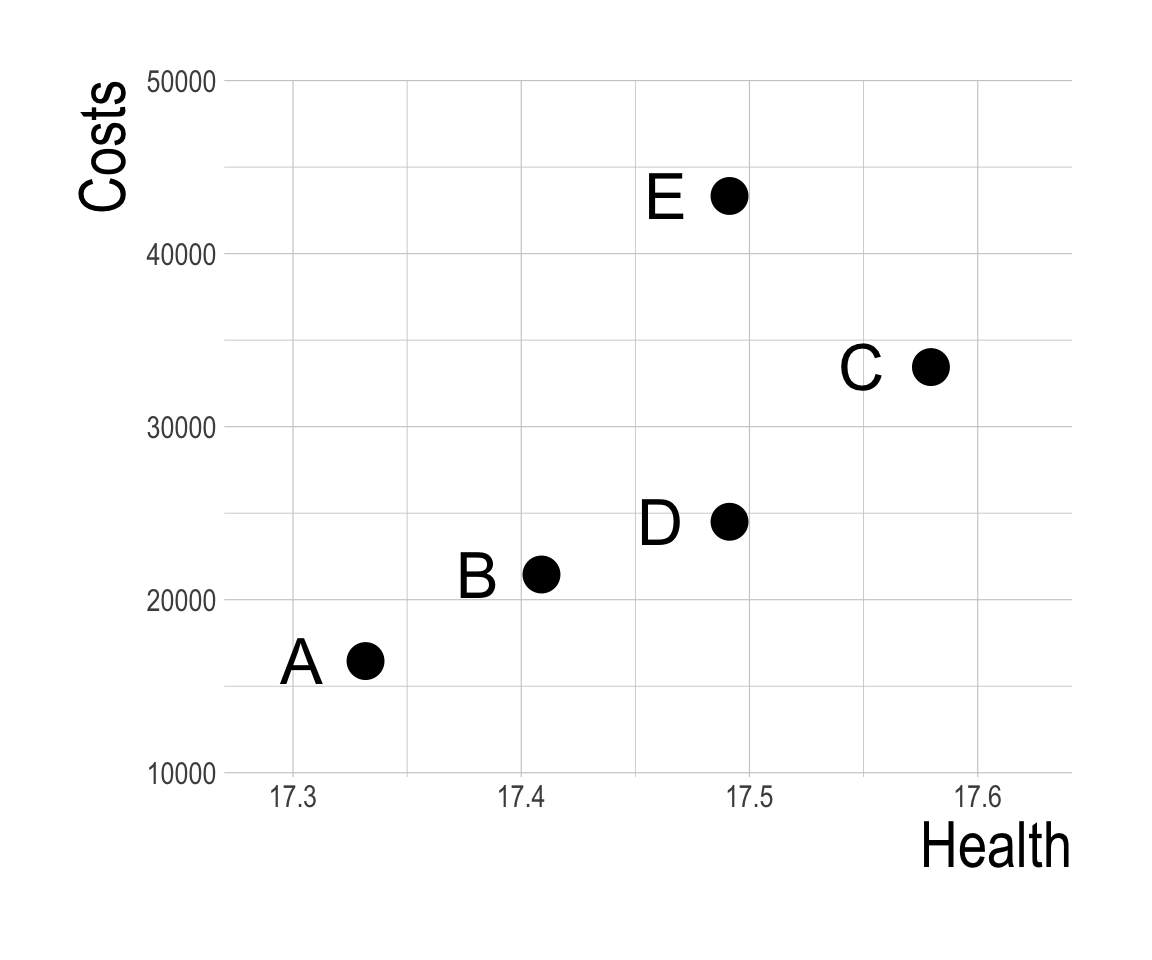
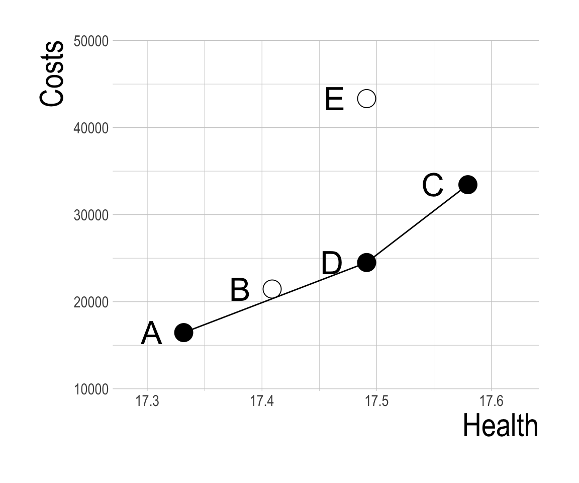
Determining Dominated Strategies
- We’re not quite done yet.
- Notice something odd about strategy B?
- It’s ICER is higher than the next most costly alternative (strategy D).
- Let’s look briefly at each strategy’s Cost and QALYs plotted in a graph.
| Strategy | Cost | dCost | QALYs | dQALYs | ICER | |
|---|---|---|---|---|---|---|
| A | 16,454 | 17.332 | ||||
| B | 21,457 | 5,002.6 | 17.409 | 0.07709 | 64,895 | |
| D | 24,504 | 3,047.5 | 17.491 | 0.08239 | 36,989 | |
| C | 33,443 | 8,939.2 | 17.580 | 0.08825 | 101,292 | |
| E | 43,332 | 17.491 |
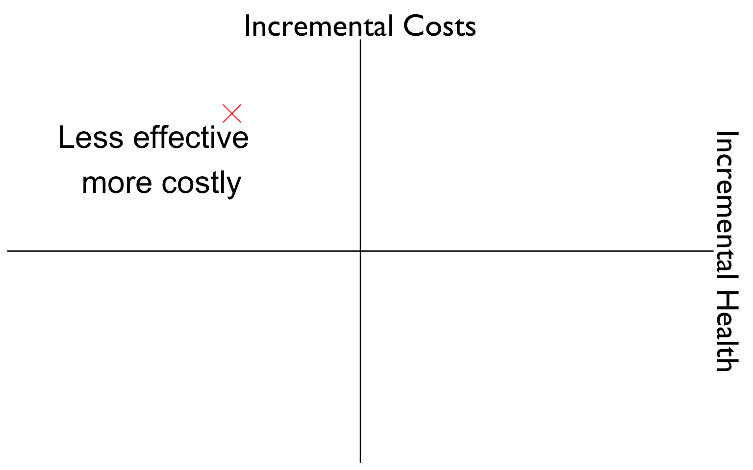
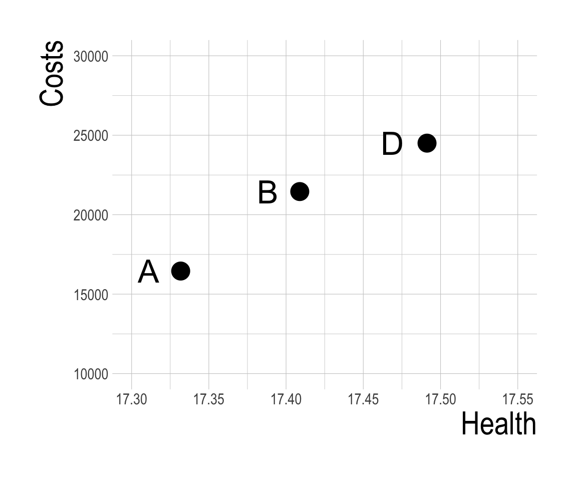
Determining Dominated Strategies
Determining Dominated Strategies
- Suppose strategy A is the status quo, and we may be willing to implement a strategy that increases health at some cost.
- Is our next best option strategy B?
- Let’s zoom in for a minute on strategies A, B, and D.

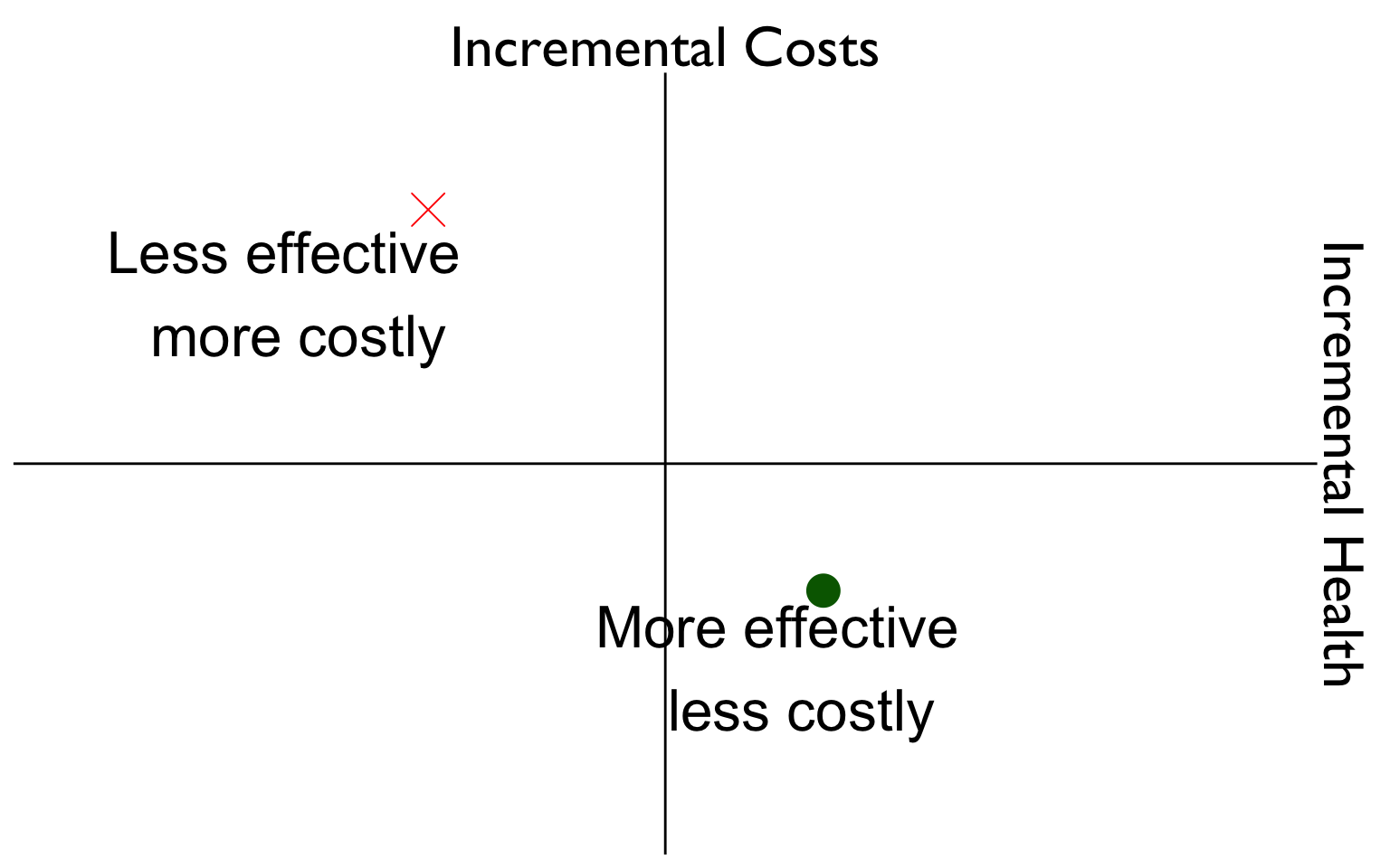
Determining Dominated Strategies
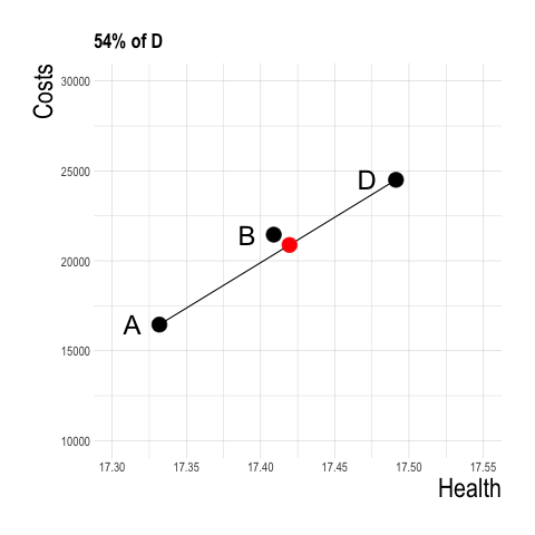
- Perhaps instead of implementing B, we could implement some fraction of strategy D and obtain better health outcomes at lower cost?
Determining Dominated Strategies
- If we partially implement strategy D (e.g., A for 99% of the population, D for 1%) we would have a strategy that falls on a line connecting A to D.
- What happens at a strategy of roughly 50% strategy A and 50% Strategy D?
Determining Dominated Strategies
- A strategy of B for 54% of the population and A for 46% of the population yields greater health benefit at lower cost than B!
- Therefore, strategy B is dominated through a concept known as extended dominance.
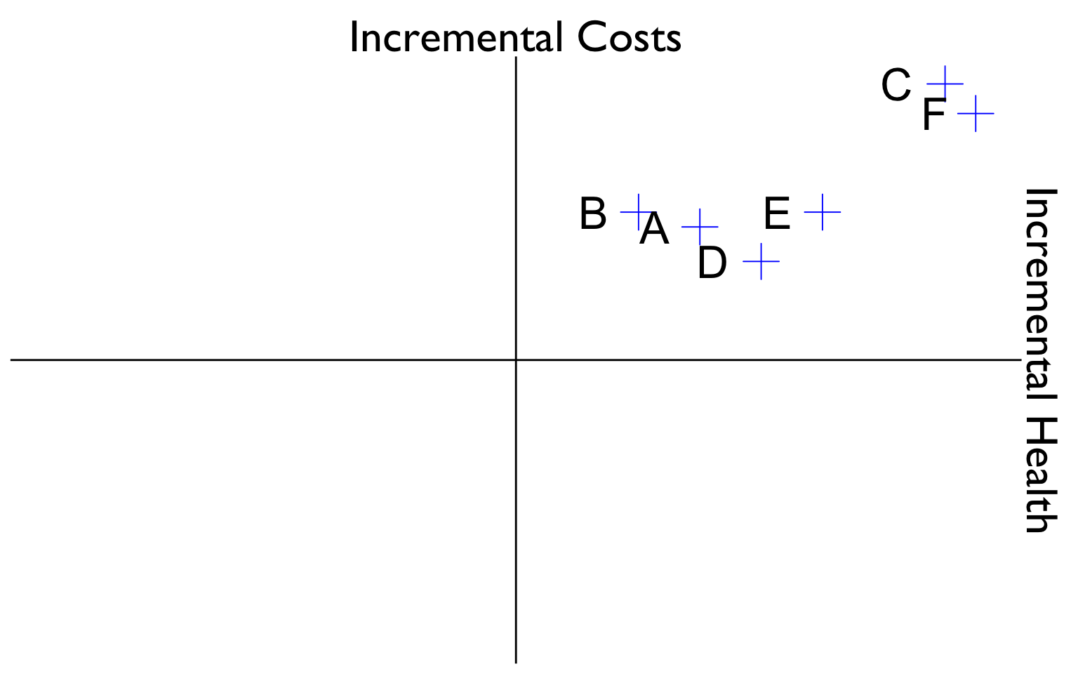
Determining Dominated Strategies
- Strategies in the interior of the cost-effectiveness frontier can be ruled out due to dominance (strong or extended)
Determining Dominated Strategies
- A telltale sign of extended dominance in a (sorted) CEA table is a strategy with a higher ICER than the next most expensive option.
| Strategy | Cost | dCost | QALYs | dQALYs | ICER | |
|---|---|---|---|---|---|---|
| A | 16,454 | 17.332 | ||||
| B | 21,457 | 5,002.6 | 17.409 | 0.07709 | 64,895 | Dominated (Extended) |
| D | 24,504 | 3,047.5 | 17.491 | 0.08239 | 36,989 | |
| C | 33,443 | 8,939.2 | 17.580 | 0.08825 | 101,292 | |
| E | 43,332 | 17.491 | Dominated |
Incremental CEA
Calculate costs and effects for each strategy.
Sort table by costs in ascending order.1
Calculate ICER based on difference in costs and effects.
Determine dominated strategies (ICER<0).
Re-calculate ICERs after eliminating dominated strategies.
6. Determine strategies ruled out by extended dominance.
| Strategy | Cost | dCost | QALYs | dQALYs | ICER | |
|---|---|---|---|---|---|---|
| A | 16,454 | 17.332 | ||||
| B | 21,457 | 5,002.6 | 17.409 | 0.07709 | 64,895 | Dominated (Extended) |
| D | 24,504 | 3,047.5 | 17.491 | 0.08239 | 36,989 | |
| C | 33,443 | 8,939.2 | 17.580 | 0.08825 | 101,292 | |
| E | 43,332 | 17.491 | Dominated |
Incremental CEA
7. Re-calculate ICERs after ruling out all dominated strategies.
| Strategy | Cost | dCost | QALYs | dQALYs | ICER | |
|---|---|---|---|---|---|---|
| A | 16,454 | 17.332 | ||||
| D | 24,504 | 8,050.1 | 17.491 | 0.15948 | 50,478 | |
| C | 33,443 | 8,939.2 | 17.580 | 0.08825 | 101,292 | |
| E | 43,332 | 17.491 | Dominated | |||
| B | 21,457 | 17.409 | Dominated (Extended) |
CEA Thresholds
- So now we have our ICERs, but how do we make a decision?
- We must define a threshold – a value that determines whether or not we implement a given strategy.
- What are common threshold and how are they determined?
CEA Thresholds
Decision should be informed by the value of what will be given up as a consequence of those cost.
- Known as the “opportunity cost.”
If resources are committed to the funding of one intervention, then they are not available to fund and deliver others.
The opportunity cost of a commitment of resources is the health forgone because these “other” interventions that are available to the health system cannot be delivered.
Source: Woods et al. (2016)
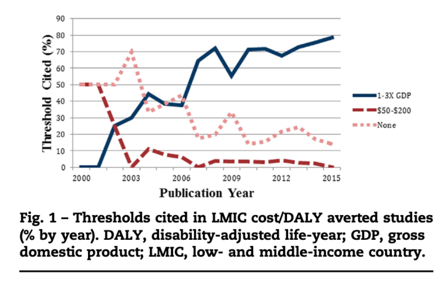
CEA Thresholds in LMICs
- WHO: intervention is “very cost-effective” if cost per DALY averted is less than GDP per capita (GDPpc).
- “Cost effective” if DALY averted is less than 3x GDPpc.
CEA Thresholds in LMICs
- Some have argued the WHO’s guidelines may be too high and result in adoption of interventions that displace existing services that provide greater health benefit.
- Suggest 0.5 GDPpc is a more appropriate benchmark for low-income countries and 0.71 GDPpc for middle-income countries.
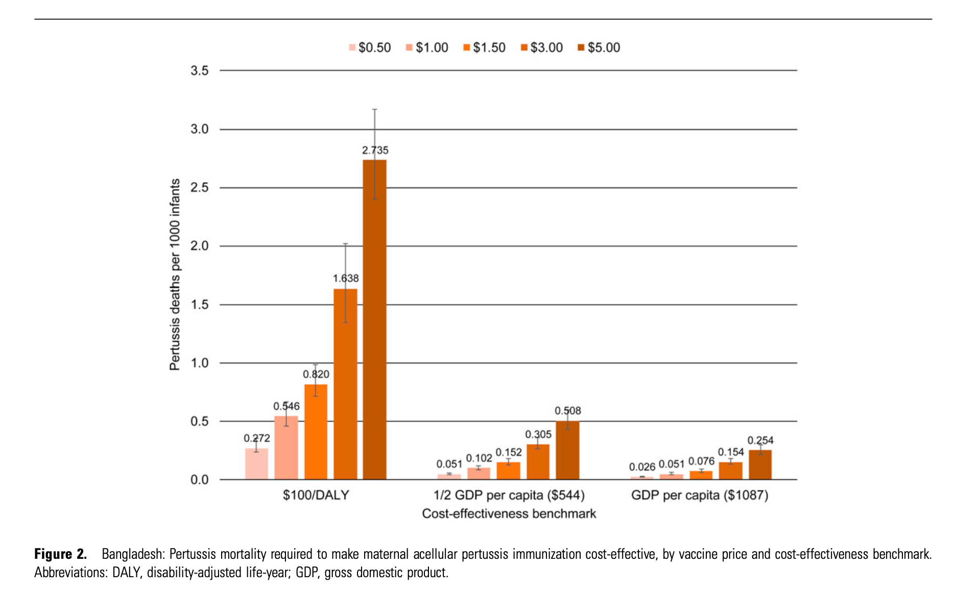
CEA Thresholds in LMICs

CEA Thresholds in LMICs
Maternal Pertussis Immunization