Case Study 3: Constructing a Transition Probability Matrix from Input Parameters
Introduction and Learning Objectives
This case study is designed to get you familiar with conducting Markov modeling in Excel. Specific learning objectives are as follows:
Parameterize and structure a Markov model.
Embed a transition probability matrix using rate-to-probability conversion formulas (Option 1) and matrix exponentiation (Option 2)
Overview of Decision Problem
Our running applied case study will examine a preventive health measure designed to protect against the onset of a disease (“sick”). Only a few of these details are relevant for completing Case Study 3, however for the sake of completeness we include them below.
- All patients start out healthy (utility weight = 1.0)
- Becoming sick reduces utility to 0.75 and carries yearly treatment costs $1000 .
- Becoming sick substantially increases the likelihood of death (Hazard Ratio =3).
- Population cohort starts at age 25 and is followed until age 100 (or everyone dies).
- Background mortality is based on life table data.
Treatment Options
The standard of care (Treatment “A”) is a preventive measure (e.g., a drug, screening program, etc.) that costs $25 per yr. However, there are several new preventive measures with varying costs and effects:
| Strategy | Cost | Hazard Ratio of Becoming Sick (Reference for HR: Strategy A) |
|---|---|---|
| A | 25 | |
| B | 1000 | 0.96 |
| C | 3100 | 0.88 |
| D | 1550 | 0.92 |
| E | 5000 | 0.92 |
Our primary decision problem, then, is to determine whether the Ministry of Health should adopt a new preventive measure.
Part 1. Parameterize the Model
You will notice that the parameters worksheet looks similar to the one in Case Study 2 (CS2), however it is a bit longer. In CS2, we provided you with the transition probabilities; in this case study you will calculate them yourself.
As before, our first step is to define variable names for all the inputs parameters in our decision problem. Again, the blog posting on useful Excel functions covers how to assign variable names in detail, and using several methods.
Use variable names to assign values to each parameter in the Excel document.
You may notice that the orange-shaded variables at the bottom do not change once we define variables for all its inputs. To fix this, in the base_case column, simply add an “=” sign to the formulas, as you did in the last case study. After doing so, the numeric value for these variables should appear.

Part 2: Fill out the Rate Matrix
Next, turn your attention to the transition matrix worksheet. There, you will see a section (labelled Part 2) where you can fill out the rate matrices for each treatment strategy.
Let’s start by filling out the rate matrix for the reference (standard of care) strategy, which is strategy A.

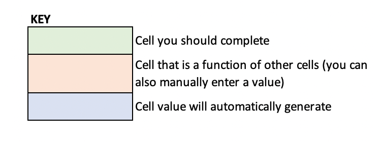
Also note the key at the bottom of the worksheet. Green cells are those you should fill out directly (using parameter names, of course!). Red cells are functions of other cells in the matrix (e.g., the diagonal of the rate matrix is just -1 times the sum of the other row elements). Blue cells will be calculated for you once the correct inputs (red and green cells) are in place.
Use your defined parameter names to fill out the rate matrix values for Strategy A. The final matrix should have numeric values (e.g., 0.15). Once the full matrix has values, define a name (m_R_A) for the matrix.
Enter zeros in the rate matrix in cells where there is no defined transition, and for the cell corresponding to the death-to-death transition rate.
For some transitions and strategies, you will need to use both the baseline rate (i.e., r_*) and a hazard ratio (i.e., hr_*) to calculate the final transition rate for the cell. For example, if the baseline rate for a hypothetical transition is 0.1 and a given strategy modifies this rate by a hazard ratio of 0.9, then the final rate for that strategy would be 0.1 * 0.9 =0.09.
Make sure to multiply each rate in the rate matrix by the time step (i.e., n_cycle_length) so you can easily convert the cycle time length if you need to!
Our next step is to finish the remaining rate matrices for strategies B through E. Note that these strategies are based on the Strategy A matrix, however some transitions are modified by a hazard rate specific to the strategy.
Fill out the rate matrix values for Strategies B through D. Then define a names (m_R_B, m_R_C, etc.) for the rate matrices.
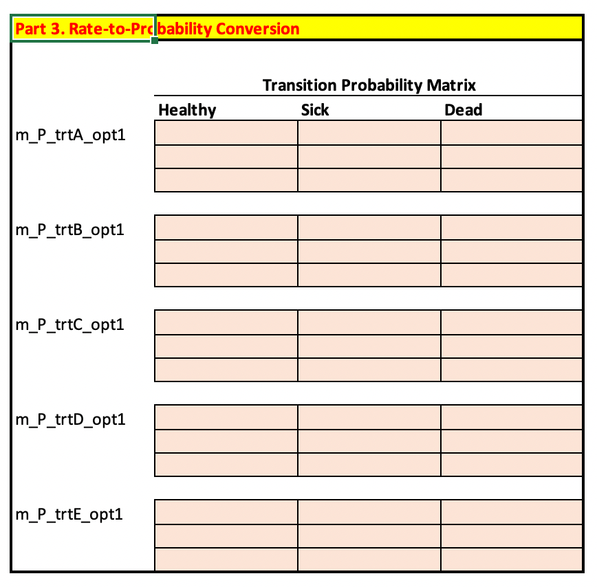
Part 3: Rate-to-Probability Conversion Formulas
With the input rates defined we will now turn our attention to converting these rates into transition probabilities. Our first option is to use the standard formulas:
\[ p_{HS}= \frac{r_{HS}}{r_{HS}+r_{HD}}\big ( 1 - e^{-(r_{HS}+r_{HD})\Delta t}\big ) \]
\[ p_{HD}= \frac{r_{HD}}{r_{HS}+r_{HD}}\big ( 1 - e^{-(r_{HS}+r_{HD})\Delta t}\big ) \]
\[ p_{HH} = e^{-(r_{HS}+r_{HD})\Delta t} \]
In the above formulas, r_* is a transition rate and \(\Delta t\) is the timestep, which in the Excel document is set to a value of 1 and stored in the variable n_cycle_length.
Use the formulas above to fill out the transition probability matrix for each strategy.
If you multiplied each rate in the transition rate matrix by the time step, you do not need to do it again here!
Be careful with the Dead-to-Dead transition probability; the rate is set to zero in the rate matrix, but this probability should be manually set to 1 in the transition probability matrix.
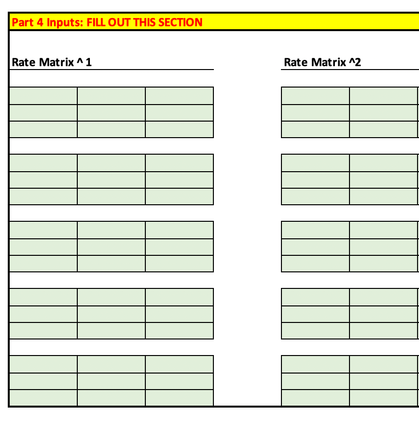
Part 4: Embedding the Transition Probability Matrix
In this section we will use an alternative approach—matrix exponentiation–to embed the transition probability matrix.
Unfortunately, Excel does not have built-in capabilities for matrix exponentiation. Fortunately, however, we can use a Taylor series expansion approach to exponentiation. The basic formula is,
\[ \exp(R) = \sum_{n=0}^{\infty}\frac{R^n}{n!} \] However in practice we will only need to take \(R\) to the fourth power to get a reasonable transition probability matrix.
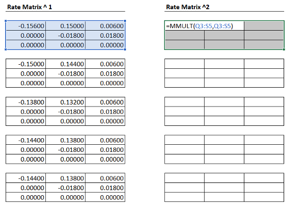
To take a matrix to a power in Excel, we can simply use the MMULT() function. For example, MMULT(R,R) is equivalent to \(R^2\).
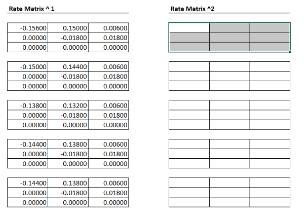
Use matrix multiplication on each rate matrix to calculate \(R^1\), \(R^2\), \(R^3\) and \(R^4\).
NOTE Depending on your Excel version, you may need to use a slightly different approach to ensure the MMULT() function executes.
First, highlight the region you want to apply matrix multiplication to:
Next, enter the formula you want to execute:
Finally, press control+shift+enter to get the formula to execute over the entire region of cells.
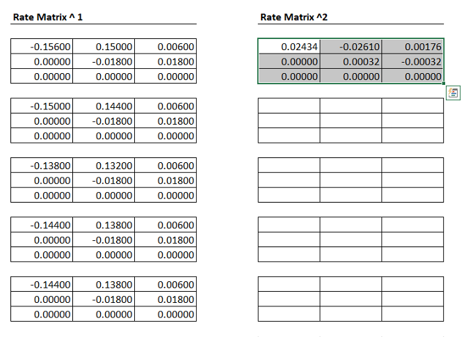
You will notice that there is a binary (identity) matrix in the Excel worksheet. This binary matrix simply reflects that \(R^0\) is an identity matrix (i.e., a matrix with 1’s in the diagonal elements, and 0 everywhere else). Also note that \(R^1=R\).
 Once you have calculated \(R^1\), \(R^2\), \(R^3\) and \(R^4\) you will notice that the transition probability matrix (with blue cells) has updated.
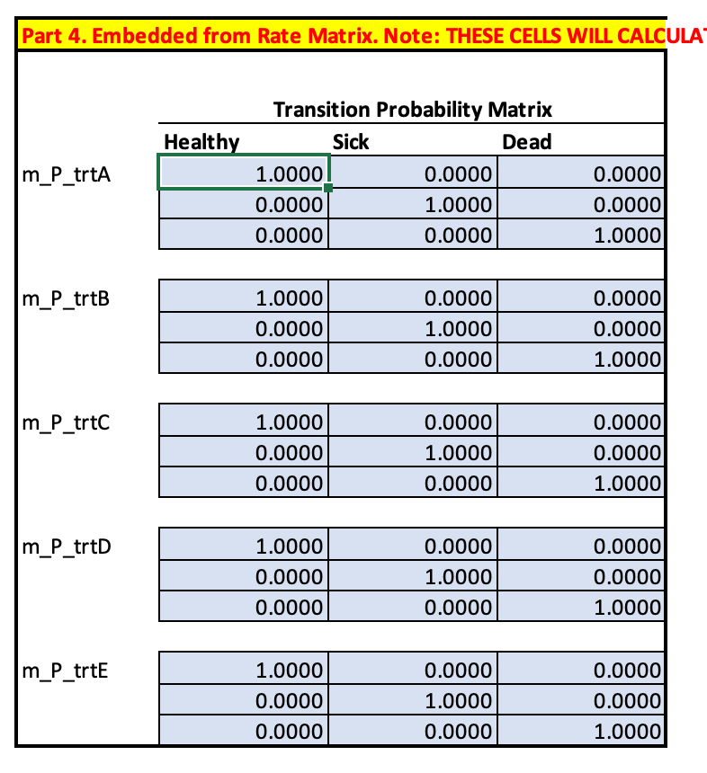
Compare the calculated transition probability matrices from Parts 3 and 4. How similar are they? For probabilities that are different, can you explain why?
Part 5: Changing the Time Step
The above exercises constructed a transition probability matrix for an annual time step (i.e., n_cycle_length=1). Now suppose that we wanted to convert to a monthly cycle instead.
Modify the model input parameters so that the timestep is monthly, rather than yearly. How do the transition probabilities change?