4. Introduction to Markov Modeling
Learning Objectives and Outline
Learning Objectives
-Discuss pros and cons of decision modeling using decision trees vs. a formal deterministic model.
-Understand the components and structure of discrete time Markov models.
-Discuss how to structure and parameterize a transition probability matrix.
-Understand how to construct a Markov trace using a transition probability matrix and state occupancy vector.
A Simple Disease Process
- Suppose we want to model the cost-effectiveness of alternative strategies to prevent a disease from occurring.
- We start with a healthy population of 25 year olds, and there are three health states people can experience:
- Remain Healthy
- Become Sick
- Death
A Simple Disease Process
- Remaining healthy carries no utility decrement (utility weight = 1.0 per cycle in healthy state)
- Becoming sick carries a 0.25 utility decrement for the remainder of the person’s life (utility weight = 0.75)
- Death carries a utility value of 0.0.
A Simple Disease Process
- There is no cost associated with remaining healthy.
- Becoming sick incurs $1,000 / year in costs.
- Becoming sick increases the risk of death by 300%.
A Simple Disease Process
The ministry of health is considering five preventive care strategies that reduce the risk of becoming sick:
| Strategy | Description | Cost |
|---|---|---|
| A | Standard of Care | $25/year |
| B | Additional 4% reduction in risk of becoming sick | $1,000/year |
| C | 12% reduction in risk | $3,100/year |
| D | 8% reduction in risk | $1,550/year |
| E | 8% reduction in risk | $5,000/year |
Model Option 1: Decision Tree
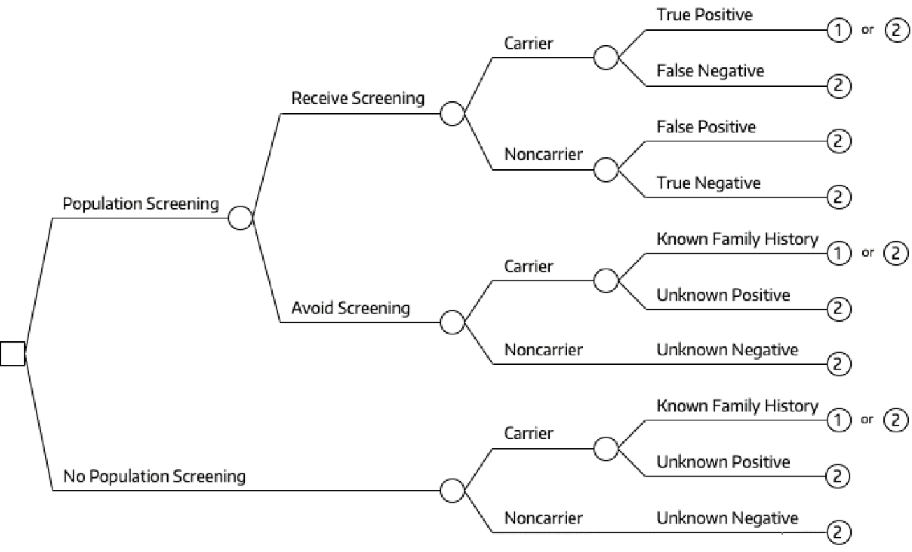
- One option would be to use a decision tree to model the expected utility and costs associated with each strategy.
Model Option 1: Decision Tree
- One option would be to use a decision tree to model the expected utility and costs associated with each strategy.
- What limitations do you see?
Decision tree for two full cycles.
Strategy A decision tree for 5 cycles.
Decision Trees
| Pros | Cons |
|---|---|
| Simple, rapid & can provide insights |
Decision Trees
| Pros | Cons |
|---|---|
| Simple, rapid & can provide insights | |
| Easy to describe & understand |
Decision Trees
| Pros | Cons |
|---|---|
| Simple, rapid & can provide insights | |
| Easy to describe & understand | |
| Works well with limited time horizon |
Decision Trees
| Pros | Cons |
|---|---|
| Simple, rapid & can provide insights | Difficult to include clinical detail |
| Easy to describe & understand | |
| Works well with limited time horizon |
Decision Trees
| Pros | Cons |
|---|---|
| Simple, rapid & can provide insights | Difficult to include clinical detail |
| Easy to describe & understand | Elapse of time is not readily evident. |
| Works well with limited time horizon |
Decision Trees
| Pros | Cons |
|---|---|
| Simple, rapid & can provide insights | Difficult to include clinical detail |
| Easy to describe & understand | Elapse of time is not readily evident. |
| Works well with limited time horizon | Difficult to model longer (>1 cycle) time horizons |
Next Steps
- Ideally we want a modeling approach that can incorporate flexibility and handle the complexities that make decision trees difficult/unwieldy.
Markov Models
Markov Models
Common approach in decision analyses that adds additional flexibility.
| Pros | Cons |
|---|---|
| Can model repeated events | |
| \(\quad \quad \quad \quad \quad \quad\) |
Markov Models
Common approach in decision analyses that adds additional flexibility.
| Pros | Cons |
|---|---|
| Can model repeated events | |
| Can model more complex + longitudinal clinical events |
Markov Models
Common approach in decision analyses that adds additional flexibility.
| Pros | Cons |
|---|---|
| Can model repeated events | |
| Can model more complex + longitudinal clinical events | |
| Not computationally intensive; efficient to model and debug |
Markov Models
The advantages of Markov models derive from the fact that they are structured around mutually exclusive disease states.
These disease states represent the possible states or consequences of strategies or options under consideration.
Because there are a fixed number of disease states the population can be in, there is no need to model complex pathways, as we saw in the decision tree “explosion” a few slides back.
Markov Trees
It is also common to pair a Markov model with a decision tree.1
Markov Trees
It is also common to pair a Markov model with a decision tree.1
Markov Tree
A simple decision tree is implicit in nearly every decision analysis.

Markov Tree: Example
Treatment A:
Constructing a Markov Model
Steps
- Define the decision problem.
- Conceptualize the model.
- Parameterize the model.
- Calculate or define the transition probability matrix.
- Run the model.
1. Define the Decision Problem
Step 1: Define the Decision Problem
We defined the decision problem earlier in this lecture, so we’ll repeat the basic objectives briefly here.
Step 1: Define the Decision Problem
Goal: model the cost-effectiveness of alternative strategies to prevent a disease from occurring.
| Strategy | Description | Cost |
|---|---|---|
| A | Standard of Care | $25/year |
| B | Additional 4% reduction in risk of becoming sick | $1,000/year |
| C | 12% reduction in risk | $3,100/year |
| D | 8% reduction in risk | $1,550/year |
| E | 8% reduction in risk | $5,000/year |
Step 1: Define the Decision Problem
2. Conceptualize the Markov Model
2. Conceptualize the Markov Model
Two major steps:
2a. Determine health states
2b. Determine transitions
Step 2: Conceptualize the Model
2a. Determine health states
- There three health states people can experience:
- Remain Healthy
- Become Sick
- Death
Step 2: Conceptualize the Model
2a. Determine health states
- There three health states people can experience:
- Remain Healthy
- Become Sick
- Death
2b. Determine transitions
- Individuals who become sick cannot transition back to healthy.
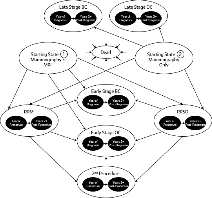
Step 2: Conceptualize the Model
Diagram constructed using the Graphviz Visual Editor
3. Parameterize the Model
3. Parameterize the Model
Basic steps
3a. Determine basic model parameters
3b. Curate and define model inputs
3. Parameterize the Model
Basic steps
3a. Determine basic model parameters
- Define the population (e.g., 25 year old females)
- Define the Markov cycle length (e.g., 1-year cycle)
- Define the time horizon (e.g., followed until age 100 or death)
3a. Define the Markov Cycle Length
- Fundamentally, we’re modeling a continuous time process (e.g., progression of disease).
- A discrete time Markov model “breaks up” time into “chunks” (i.e., “cycles”).
- A consequence is that the model will show us what fraction start out a cycle in a given state, and what fraction end up in each state at the end of the cycle.
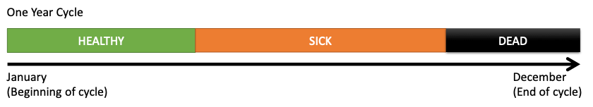
3a. Define the Markov cycle length
- Suppose we used a one-year cycle for the healthy-sick-dead model.
- Think about the underlying (continuous time) disease process.
- Recall that becoming sick substantially increases the likelihood of death.
- If we’re not careful, what are we (implicitly) assuming can and can’t happen in a single cycle?
3a. Define the Markov Cycle Length
3a. Define the Markov Cycle Length
The challenge of selecting an appropriate cycle length boils down to how we deal with competing risks.
- Competing risks: individuals can transition from their current health state to two or more other health states.
3a. Define the Markov Cycle Length
The challenge of selecting an appropriate cycle length boils down to how we deal with competing risks.
- If we’re not careful, we could effectively rule out the possibility of Healthy Sick Dead within a cycle.
- The model would look like a basic Healthy Dead transition, but they took a detour through Sick along the way!
3a. Define the Markov Cycle Length
| Pros | Cons |
|---|---|
| Can model repeated events | Competing risks are a challenge |
| Can model more complex + longitudinal clinical events | |
| Not computationally intensive; efficient to model and debug |
3a. Define the Markov Cycle Length
- It may be tempting to simply shorten the cycle length (e.g., use 1 day cycle vs. 1 year cycle).
- For a 75 year horizon, how many cycles would that be?
- 27,375!!!
- Any possible issues with this?
3a. Define the Markov Cycle Length
- Shortening the cycle creates a computational challenge.
- Base case requires 27,375 daily cycles.
- Now suppose we want to run 2,000 probabilistic sensitivity analysis model runs.
- We now have 57,750,000 cycle runs to contend with!
3a. Define the Markov Cycle Length
| Pros | Cons |
|---|---|
| Can model repeated events | Can only transition once in a given cycle |
| Can model more complex + longitudinal clinical events | Shortening the cycle can create computational challenges. |
| Not computationally intensive; efficient to model and debug |
3a. Define the Markov Cycle Length
More challenges …
- If our model has tunnel states (we’ll get to these in a later lecture) we can quickly run into additional “state explosion” issues.
- A one-year tunnel state would require 365 daily tunnel states with a daily cycle …
3a. Define the Markov Cycle Length
| Pros | Cons |
|---|---|
| Can model repeated events | Can only transition once in a given cycle |
| Can model more complex + longitudinal clinical events | Shortening the cycle can create computational challenges. |
| Not computationally intensive; efficient to model and debug | Shortening cycle can cause “state explosion” if tunnel states are used |
3a. Define the Markov Cycle Length
- It’s also advisable to pick a cycle length that aligns with the clinical/disease timelines of the decision problem.
- Treatment schedules.
- Acute vs. chronic condition.
- Another option is to incorporate “short-run” events that happen early in the course of a disease/intervention within the decision tree, then allow the Markov model to model longer-term health consequences.
3a. Define the Markov Cycle Length
- We will show you an approach to embedding a transition probability matrix that avoids many of these problems.
- The “cost” of this approach is that you need to (slightly!) restructure your model to include some non-Markovian elements in the transition matrix.
- More details will come in a later lecture!
3. Parameterize the Model
3b. Curate and define model inputs
3b.i. Source and define the base case values.
3b.ii. Source and define sources of uncertainty.
Please note that future lectures will give you specific further guidance on sources and strategies for 3b.i. and 3b.ii!!
3. Parameterize the Model
3b. Curate and define model inputs
- Rate of disease onset
- Health state utilities and costs
- Hazard ratios, odds ratios or relative risks for different strategies.
- … and so on.
3. Parameterize the Model
We defined many of the underlying parameters earlier in this lecture, so we’ll repeat them briefly here.
3. Parameterize the Model
- We start with a healthy population of 25 year olds and follow them until age 100 (or death, if earlier).
- Remaining healthy carries no utility decrement (utility weight= 1.0)
- Becoming sick carries a 0.25 utility decrement for the remainder of the person’s life (utility weight = 0.75)
- Death carries a utility weight value of 0.0.
3. Parameterize the Model
- There is no cost associated with remaining healthy.
- Becoming sick incurs $1,000 / year in costs.
- Becoming sick increases the risk of death by 300%.
3. Parameterize the Model
Each strategy has a different cost and impact on the likelihood of becoming sick.
| Strategy | Description | Cost |
|---|---|---|
| A | Standard of Care | $25/year |
| B | Additional 4% reduction in risk of becoming sick | $1,000/year |
| C | 12% reduction in risk | $3,100/year |
| D | 8% reduction in risk | $1,550/year |
| E | 8% reduction in risk | $5,000/year |
3. Parameterize the Model
It is critical to follow a formal process for parameterizing your model.
- Often, parameters are drawn from the published literature, and it is important to track the source (published value, assumption, etc.) for each model parameter.
- For example, the percent risk reduction parameter for each strategy may come from different clinical trials.
- The parameter governing death from background causes may be derived from mortality data.
3. Parameterize the Model
It is critical to follow a formal process for parameterizing your model.
- Some parameters may just be values (e.g., cost of Strategy A is $25/yr)
- Some parameters may be functions of other parameters.
- For example, suppose we want to follow a cohort of 25 year olds until age 100 or death, if it occurs earlier.
- In that case we have two “fixed” parameters: the starting age, and the maximum age.
- We can use these two parameters to infer the total number of cycles we need to run.
3. Parameterize the Model
It is critical to follow a formal process for parameterizing your model.
- Parameters also have various “flavors”:
- Probabilities
- Rates
- Hazard ratios
- Costs
- Utilities
- etc.
3. Parameterize the Model
It is critical to follow a formal process for parameterizing your model.
All of the above highlight the importance of adopting a formal process for naming and tracking the value, source, and uncertainty distribution of all model parameters in one place.
We recommend a structured approach based on parameter naming conventions and parameter tables.
3. Parameterize the Model
Naming conventions:
| type | prefix |
|---|---|
| Probability | p_ |
| Rate | r_ |
| Matrix | m_ |
| Cost | c_ |
| Utility | u_ |
| Hazard Ratio | hr_ |
Parameter Table
Note: Only a subset of model parameters are shown in table.
| Parameter Table | ||||||
| param | base_case | formula | description | notes | distribution | source |
|---|---|---|---|---|---|---|
| n_age_init | 25.00 | Age at baseline | Modeling Parameter | |||
| n_age_max | 100.00 | Maximum age of followup | Modeling Parameter | |||
| u_H | 1.00 | Utility weight of healthy (H) | beta(shape1 = 200, shape2 = 3) | Leech et al. (2022) | ||
| u_S | 0.75 | Utility weight of sick (S) | beta(shape1 = 130, shape2 = 45) | Leech et al. (2022) | ||
| c_S | 1000.00 | Annual cost of sick (S) | gamma(shape = 44.4, scale = 22.5) | Graves et al. (2022) | ||
| c_trtA | 25.00 | Cost of treatment A | gamma(shape = 12.5, scale = 2) | Martin et al. (2022) | ||
| c_trtB | 1000.00 | Cost of treatment B | gamma(shape = 12, scale = 83.3) | Assumption | ||
| c_trtC | 3100.00 | Cost of treatment C | gamma(shape = 36.144, scale = 83) | Assumption | ||
| n_cycles | 75.00 | (n_age_max - n_age_init) | Time horizon | |||
param column is the short name of the parameter
Note: Only a subset of model parameters are shown in table.
| Parameter Table | ||||||
| param | base_case | formula | description | notes | distribution | source |
|---|---|---|---|---|---|---|
| n_age_init | 25.00 | Age at baseline | Modeling Parameter | |||
| n_age_max | 100.00 | Maximum age of followup | Modeling Parameter | |||
| u_H | 1.00 | Utility weight of healthy (H) | beta(shape1 = 200, shape2 = 3) | Leech et al. (2022) | ||
| u_S | 0.75 | Utility weight of sick (S) | beta(shape1 = 130, shape2 = 45) | Leech et al. (2022) | ||
| c_S | 1000.00 | Annual cost of sick (S) | gamma(shape = 44.4, scale = 22.5) | Graves et al. (2022) | ||
| c_trtA | 25.00 | Cost of treatment A | gamma(shape = 12.5, scale = 2) | Martin et al. (2022) | ||
| c_trtB | 1000.00 | Cost of treatment B | gamma(shape = 12, scale = 83.3) | Assumption | ||
| c_trtC | 3100.00 | Cost of treatment C | gamma(shape = 36.144, scale = 83) | Assumption | ||
| n_cycles | 75.00 | (n_age_max - n_age_init) | Time horizon | |||
base_case is the parameter value for the base case.
Note: Only a subset of model parameters are shown in table.
| Parameter Table | ||||||
| param | base_case | formula | description | notes | distribution | source |
|---|---|---|---|---|---|---|
| n_age_init | 25.00 | Age at baseline | Modeling Parameter | |||
| n_age_max | 100.00 | Maximum age of followup | Modeling Parameter | |||
| u_H | 1.00 | Utility weight of healthy (H) | beta(shape1 = 200, shape2 = 3) | Leech et al. (2022) | ||
| u_S | 0.75 | Utility weight of sick (S) | beta(shape1 = 130, shape2 = 45) | Leech et al. (2022) | ||
| c_S | 1000.00 | Annual cost of sick (S) | gamma(shape = 44.4, scale = 22.5) | Graves et al. (2022) | ||
| c_trtA | 25.00 | Cost of treatment A | gamma(shape = 12.5, scale = 2) | Martin et al. (2022) | ||
| c_trtB | 1000.00 | Cost of treatment B | gamma(shape = 12, scale = 83.3) | Assumption | ||
| c_trtC | 3100.00 | Cost of treatment C | gamma(shape = 36.144, scale = 83) | Assumption | ||
| n_cycles | 75.00 | (n_age_max - n_age_init) | Time horizon | |||
formula defines model parameter formulas for parameters that are functions of other model parameters.
Note: Only a subset of model parameters are shown in table.
| Parameter Table | ||||||
| param | base_case | formula | description | notes | distribution | source |
|---|---|---|---|---|---|---|
| n_age_init | 25.00 | Age at baseline | Modeling Parameter | |||
| n_age_max | 100.00 | Maximum age of followup | Modeling Parameter | |||
| u_H | 1.00 | Utility weight of healthy (H) | beta(shape1 = 200, shape2 = 3) | Leech et al. (2022) | ||
| u_S | 0.75 | Utility weight of sick (S) | beta(shape1 = 130, shape2 = 45) | Leech et al. (2022) | ||
| c_S | 1000.00 | Annual cost of sick (S) | gamma(shape = 44.4, scale = 22.5) | Graves et al. (2022) | ||
| c_trtA | 25.00 | Cost of treatment A | gamma(shape = 12.5, scale = 2) | Martin et al. (2022) | ||
| c_trtB | 1000.00 | Cost of treatment B | gamma(shape = 12, scale = 83.3) | Assumption | ||
| c_trtC | 3100.00 | Cost of treatment C | gamma(shape = 36.144, scale = 83) | Assumption | ||
| n_cycles | 75.00 | (n_age_max - n_age_init) | Time horizon | |||
description provides a text description of the parameter.
| Parameter Table | ||||||
| param | base_case | formula | description | notes | distribution | source |
|---|---|---|---|---|---|---|
| n_age_init | 25.00 | Age at baseline | Modeling Parameter | |||
| n_age_max | 100.00 | Maximum age of followup | Modeling Parameter | |||
| u_H | 1.00 | Utility weight of healthy (H) | beta(shape1 = 200, shape2 = 3) | Leech et al. (2022) | ||
| u_S | 0.75 | Utility weight of sick (S) | beta(shape1 = 130, shape2 = 45) | Leech et al. (2022) | ||
| c_S | 1000.00 | Annual cost of sick (S) | gamma(shape = 44.4, scale = 22.5) | Graves et al. (2022) | ||
| c_trtA | 25.00 | Cost of treatment A | gamma(shape = 12.5, scale = 2) | Martin et al. (2022) | ||
| c_trtB | 1000.00 | Cost of treatment B | gamma(shape = 12, scale = 83.3) | Assumption | ||
| c_trtC | 3100.00 | Cost of treatment C | gamma(shape = 36.144, scale = 83) | Assumption | ||
| n_cycles | 75.00 | (n_age_max - n_age_init) | Time horizon | |||
Note: Only a subset of model parameters are shown in table.
notes is an optional column where you add additional notes or context for the parameter.
Note: Only a subset of model parameters are shown in table.
| Parameter Table | ||||||
| param | base_case | formula | description | notes | distribution | source |
|---|---|---|---|---|---|---|
| n_age_init | 25.00 | Age at baseline | Modeling Parameter | |||
| n_age_max | 100.00 | Maximum age of followup | Modeling Parameter | |||
| u_H | 1.00 | Utility weight of healthy (H) | beta(shape1 = 200, shape2 = 3) | Leech et al. (2022) | ||
| u_S | 0.75 | Utility weight of sick (S) | beta(shape1 = 130, shape2 = 45) | Leech et al. (2022) | ||
| c_S | 1000.00 | Annual cost of sick (S) | gamma(shape = 44.4, scale = 22.5) | Graves et al. (2022) | ||
| c_trtA | 25.00 | Cost of treatment A | gamma(shape = 12.5, scale = 2) | Martin et al. (2022) | ||
| c_trtB | 1000.00 | Cost of treatment B | gamma(shape = 12, scale = 83.3) | Assumption | ||
| c_trtC | 3100.00 | Cost of treatment C | gamma(shape = 36.144, scale = 83) | Assumption | ||
| n_cycles | 75.00 | (n_age_max - n_age_init) | Time horizon | |||
distribution specifies the uncertainty distribution for the parameter. It is used for probabilistic sensitivity analyses, which we will cover in a future lecture.
Note: Only a subset of model parameters are shown in table.
| Parameter Table | ||||||
| param | base_case | formula | description | notes | distribution | source |
|---|---|---|---|---|---|---|
| n_age_init | 25.00 | Age at baseline | Modeling Parameter | |||
| n_age_max | 100.00 | Maximum age of followup | Modeling Parameter | |||
| u_H | 1.00 | Utility weight of healthy (H) | beta(shape1 = 200, shape2 = 3) | Leech et al. (2022) | ||
| u_S | 0.75 | Utility weight of sick (S) | beta(shape1 = 130, shape2 = 45) | Leech et al. (2022) | ||
| c_S | 1000.00 | Annual cost of sick (S) | gamma(shape = 44.4, scale = 22.5) | Graves et al. (2022) | ||
| c_trtA | 25.00 | Cost of treatment A | gamma(shape = 12.5, scale = 2) | Martin et al. (2022) | ||
| c_trtB | 1000.00 | Cost of treatment B | gamma(shape = 12, scale = 83.3) | Assumption | ||
| c_trtC | 3100.00 | Cost of treatment C | gamma(shape = 36.144, scale = 83) | Assumption | ||
| n_cycles | 75.00 | (n_age_max - n_age_init) | Time horizon | |||
Note: Only a subset of model parameters are shown in table.
source provides the source for the parameter. It could be a published research article, an assumption, or just simply an unsourced modeling parameter (e.g., the starting age of the modeled cohort).
| Parameter Table | ||||||
| param | base_case | formula | description | notes | distribution | source |
|---|---|---|---|---|---|---|
| n_age_init | 25.00 | Age at baseline | Modeling Parameter | |||
| n_age_max | 100.00 | Maximum age of followup | Modeling Parameter | |||
| u_H | 1.00 | Utility weight of healthy (H) | beta(shape1 = 200, shape2 = 3) | Leech et al. (2022) | ||
| u_S | 0.75 | Utility weight of sick (S) | beta(shape1 = 130, shape2 = 45) | Leech et al. (2022) | ||
| c_S | 1000.00 | Annual cost of sick (S) | gamma(shape = 44.4, scale = 22.5) | Graves et al. (2022) | ||
| c_trtA | 25.00 | Cost of treatment A | gamma(shape = 12.5, scale = 2) | Martin et al. (2022) | ||
| c_trtB | 1000.00 | Cost of treatment B | gamma(shape = 12, scale = 83.3) | Assumption | ||
| c_trtC | 3100.00 | Cost of treatment C | gamma(shape = 36.144, scale = 83) | Assumption | ||
| n_cycles | 75.00 | (n_age_max - n_age_init) | Time horizon | |||
4. Calculate or Define the Transition Probability Matrix
Transition Probability Matrix
| Healthy | Sick | Dead | |
|---|---|---|---|
| Healthy | 0.856 | 0.138 | 0.007 |
| Sick | 0 | 0.982 | 0.02 |
| Dead | 0 | 0 | 1 |
Transition Probability Matrix
- It is rarely the case that you will have access to all necessary transition probabilities.
- Often, you will curate or define various quantities (e.g., rates, hazard rates, etc.) to construct the transition probability matrix for each strategy under consideration.
4. Calculate or Define the Transition Probability Matrix
4a. Define transition rates for each strategy.
- Often these are in your list of parameters.
- We’ll show you how to calculate these in a later lecture.
4. Calculate or Define the Transition Probability Matrix
4a. Define transition rates for each strategy.
4b. Calculate the transition probability matrix.
- We’ll show you how to calculate these in a later lecture.
4. Run the Model
Executing the model requires two inputs
Health State Occupancy at Beginning of Cycle
Transition Probability Matrix
Health State Occupancy at Beginning of Cycle
Transition Probability Matrix
Health State Occupancy at Beginning of Cycle
Transition Probability Matrix
\(\quad \quad \quad \quad \quad \quad \quad \quad\)
\(s =\)
 H S D
 1 0 0
\(P =\)
      H     S     D
H 0.856 0.138 0.007
S 0.000 0.982 0.018
D 0.000 0.000 1.000
\(\quad \quad \quad \quad\)
Health State Occupancy at Beginning of Cycle
Transition Probability Matrix
Health State Occupancy at End of Cycle
\(s =\)
 H S D
 1 0 0
\(P =\)
      H     S     D
H 0.856 0.138 0.007
S 0.000 0.982 0.018
D 0.000 0.000 1.000
\(s \cdot P=\)
     H     S     D
 0.856 0.138 0.007
Health State Occupancy at Beginning of Cycle
Transition Probability Matrix
Health State Occupancy at End of Cycle
\(s =\)
 H S D
 1 0 0
\(P =\)
      H     S     D
H 0.856 0.138 0.007
S 0.000 0.982 0.018
D 0.000 0.000 1.000
\(s \cdot P=\)
     H     S     D
 0.856 0.138 0.007
Health State Occupancy at Beginning of Cycle
Transition Probability Matrix
Health State Occupancy at End of Cycle
\(s =\)
 H S D
 1 0 0
H S D
0.856 0.138 0.007\(P =\)
H S D
H 0.856 0.138 0.007
S 0.000 0.982 0.018
D 0.000 0.000 1.000 H S D
H 0.856 0.138 0.007
S 0.000 0.982 0.018
D 0.000 0.000 1.000\(s \cdot P=\)
     H     S     D
0.856 0.138 0.007 H S D
0.733 0.254 0.015Health State Occupancy at Beginning of Cycle
Transition Probability Matrix
Health State Occupancy at End of Cycle
\(s =\)
H S D
1 0 0 H S D
0.856 0.138 0.007 H S D
0.733 0.254 0.015\(P =\)
      H     S     D
H 0.856 0.138 0.007
S 0.000 0.982 0.018
D 0.000 0.000 1.000
H S D
H 0.856 0.138 0.007
S 0.000 0.982 0.018
D 0.000 0.000 1.000 H S D
H 0.856 0.138 0.007
S 0.000 0.982 0.018
D 0.000 0.000 1.000\(s \cdot P=\)
     H     S     D
 0.856 0.138 0.007
H S D
0.733 0.254 0.015 H S D
0.627 0.35 0.025Health State Occupancy at End of Cycle
     H     S     D
 0.856 0.138 0.007
H S D
0.73274 0.25364 0.015476 H S D
0.62722 0.3502 0.025171Markov Trace
Health State Occupancy Over Ten Cycles
 cycle       H       S        D
     0 1.00000 0.00000 0.000000
     1 0.85600 0.13800 0.007000
     2 0.73274 0.25364 0.015476
     3 0.62722 0.35020 0.025171
     4 0.53690 0.43045 0.035865
     5 0.45959 0.49679 0.047371
     6 0.39341 0.55127 0.059531
     7 0.33676 0.59564 0.072207
     8 0.28826 0.63139 0.085286
     9 0.24675 0.65981 0.098669
    10 0.21122 0.68198 0.112273