Group Case Study 6: Probabilistic Sensitivity Analysis
Introduction
This group case study is designed to walk you through the following processes:
- Construct and and run a probabilistic sesitivity analysis in Excel.
- Calculate and plot a cost-effectiveness acceptibility curve for each strategy.
- Calculate and plot the cost-effectivenesss acceptibility frontier for the decision problem.
Step 1: Construct and Run a PSA
1a. Our first step is to structure our parameters worksheet to occomodate a PSA. To do this we must
Create a new parameter,
psathat is 1 if we are running the PSA and 0 if we are not. This ensures that the model uses parameter values drawn from their uncertainty distribution, rather than values set at their baseline or “base case” values, as we would do for our primary results.Create a new column called
probabilistic valuethat will contain the value drawn from the uncertainty distribution.

1b. Our next step is to draw values for each uncertain parameter and place this value in the probabilistic value column.
- For this you will use the inverse transform method discussed in the lecture.
Step 2: Structure and run the PSA
Now we navigate to the PSA worksheet to structure and run the PSA.
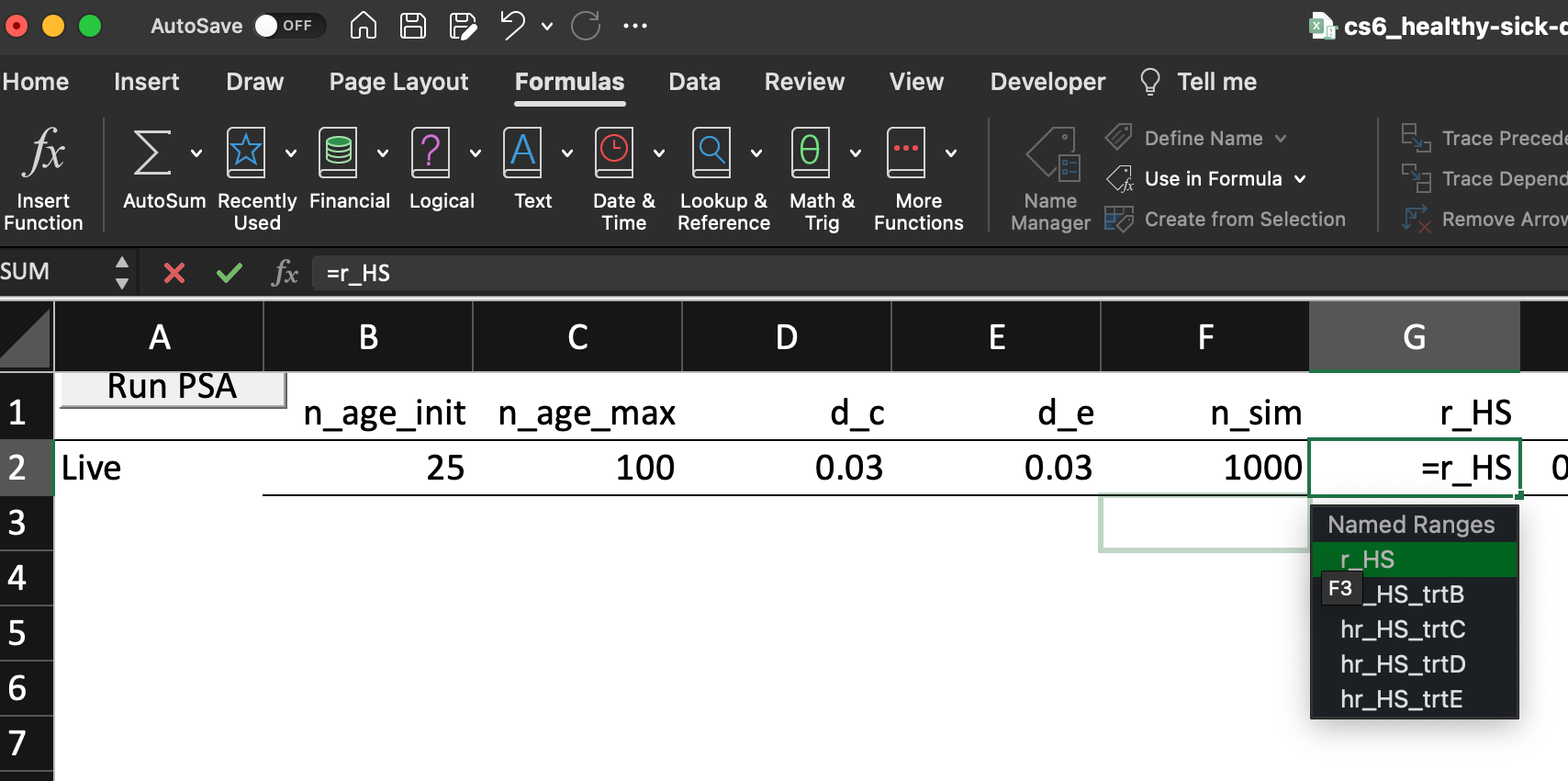
2a. Copy the “live values” to the top of the PSA worksheet.
In the top row of the
PSAworksheet you will find all the parameter names listed in theparametersworksheet.Below that, you simply provide the “live” value of the parameter in the model.
Next, we also include relevant model outputs:
- Total discounted costs for each strategy.
- Total discounted QALYs/DALYs for each strategy.

2b. Run the PSA
We have provided the following visual basic code for you to run a PSA. Essentially, all this code does is draw new values from the uncertain values and record the various outcomes calculated with those values. It does this for as many times as we specficy in the n_sim parameter, i.e., the total number of PSA runs.
Sub runPSA()

Range("parameters!psa").Value2 = 1
Application.Calculation = xlCalculationManual
Application.ScreenUpdating = False

Dim i As Integer
Dim N As Integer

N = Range("parameters!n_sim").Value2

For i = 1 To N
  Application.Calculate

  Application.StatusBar = "Reached iteration" & i

  Sheets("PSA").Cells(i + 2, 1).Value2 = i
  Sheets("PSA").Range("$B$2:$AI$2").Offset(i, 0).Value2 = Sheets("PSA").Range("$B$2:$AI$2").Value2

Next i
Application.Calculation = xlCalculationAutomatic
Application.ScreenUpdating = True
Range("parameters!psa").Value2 = 0

End Sub
You can run the PSA by navigating to the PSA worksheet and clicking the button.

Or you can simply run the macro from the Developer pane:

This will take several minutes to run, but you can find a tracker for which PSA run the macros is on the bottom left.
Once complete, you should now have PSA results!

Step 3. Construct a CEAC and CEAF
3a. Construct the CEAC Data
- Define a WTP value. Let’s start with 50,000.
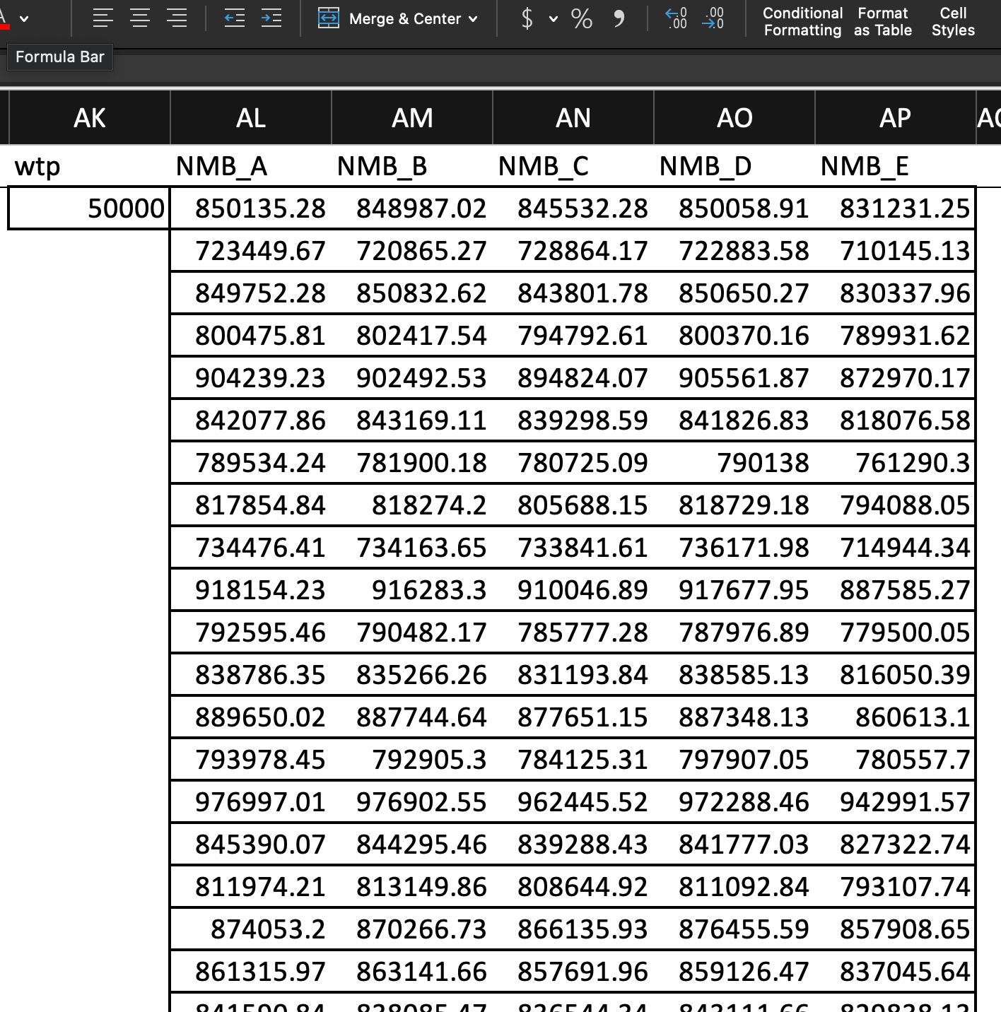
- Calculate the net monetary benefit for each strategy.
Net Monetary Benefit
\[ TOTQALY * \lambda - TOTCOST \]
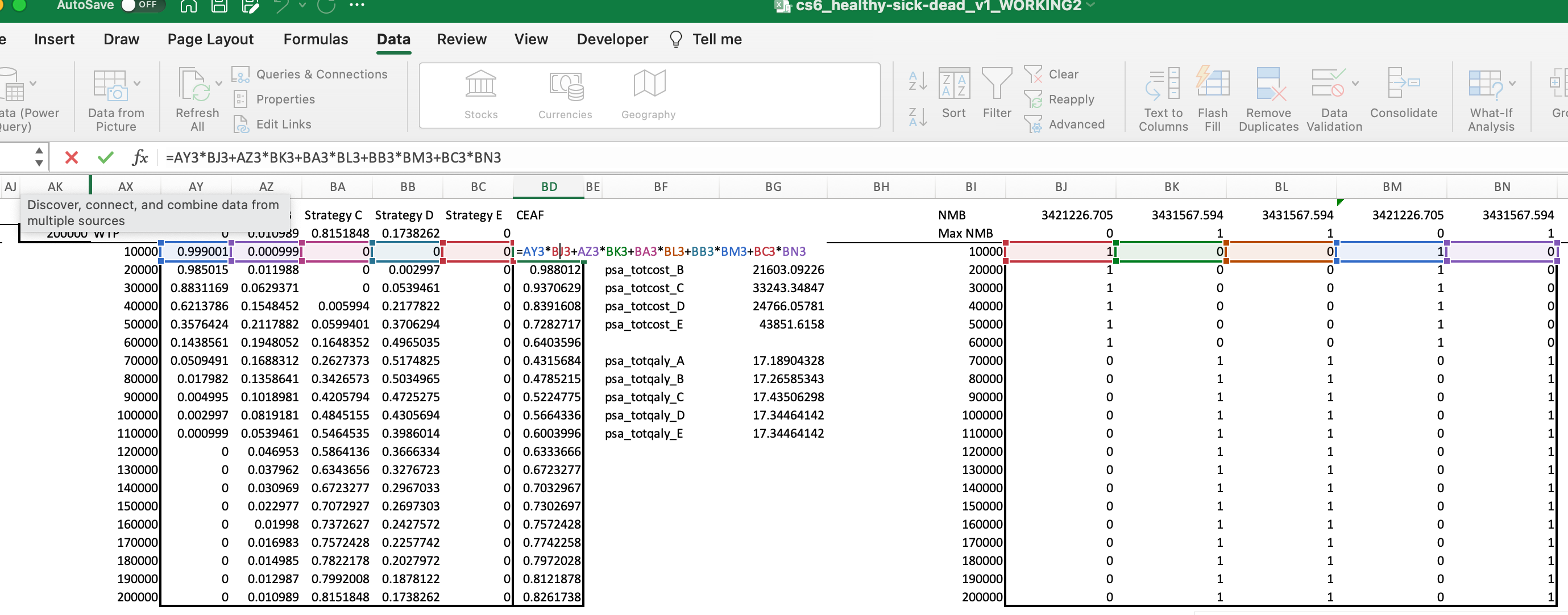
You can see these calculations for the first several PSA results below:
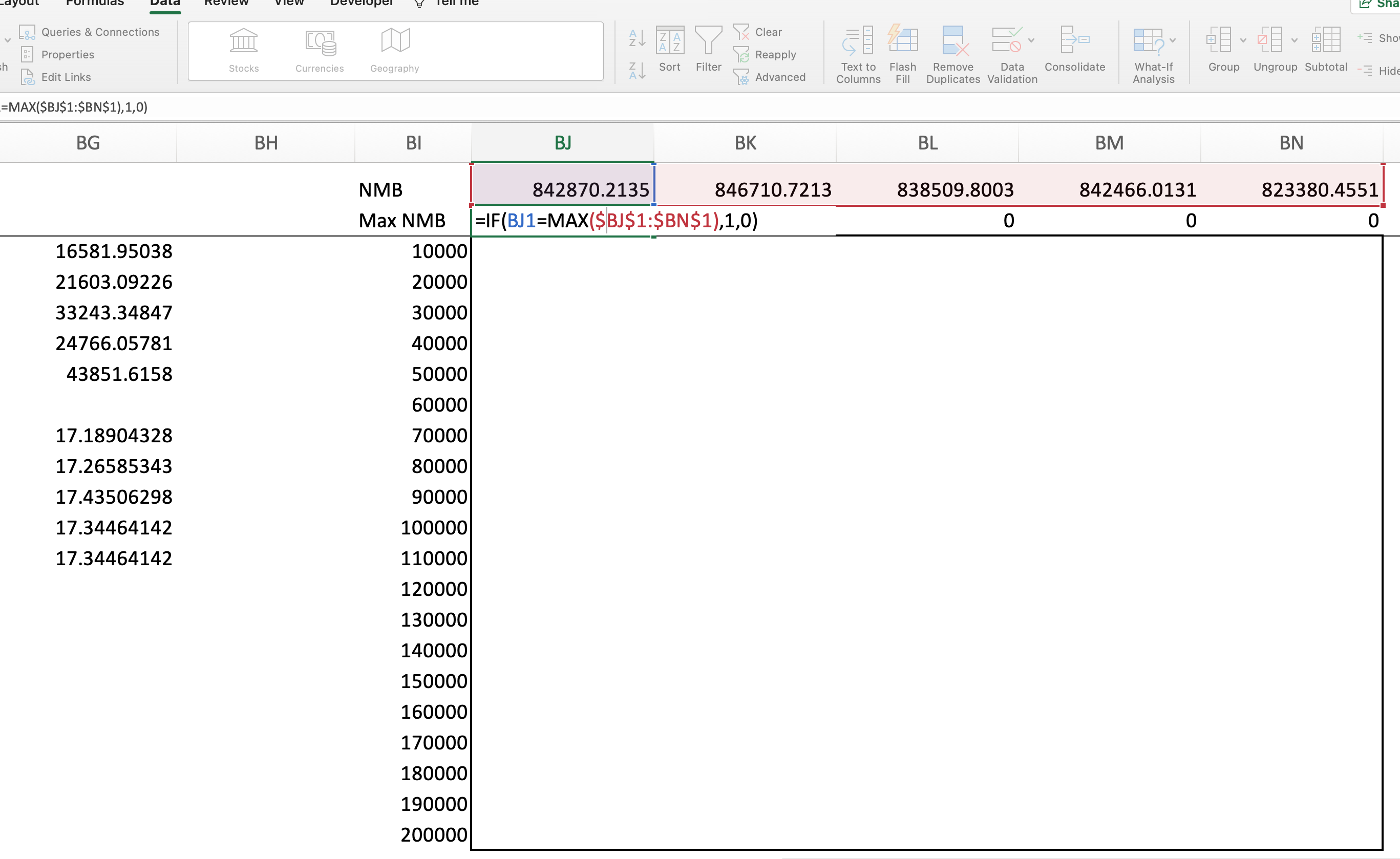
- For each iteration, determine which strategy maximizes NMB/NHB. For a given PSA iteration, you can set the value for the strategy with the MAX NMB to 1, and others to 0:

- How often is each strategy optimal? You can calculate this as the average of the binary indicator created in step 3 across all PSA model runs. This average is the fraction of the time each strategy is optimal for the given value of \(\lambda\) (i.e., 50,000/QALY).

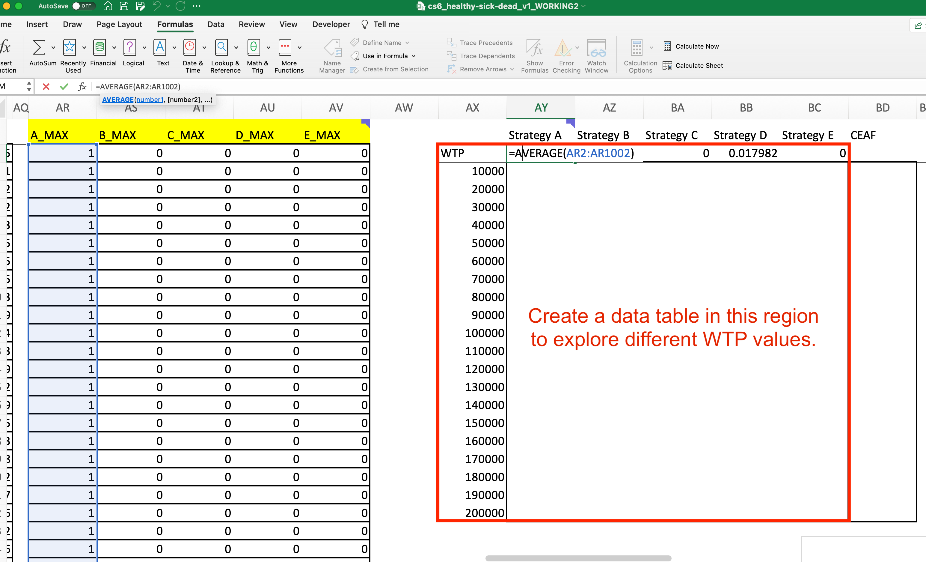
- Now we want to repeat this exercise for multiple WTP values. You can do this using a Data Table.
Now we have enough information constructed to create a cost-effectiveness acceptability curve! Before we plot it, however, we will first construct information for the cost-effectiveness acceptability frontier.
3b. Construct the CEAF Data
Our next step is to construct the data we need to plot the cost-effectiveness accectability frontier. Recall that the CEEAF shows the probability that the optimal option is cost-effective at different \(\lambda\) values.
Determine average costs and QALY* for each strategy across all PSA iterations. To do this, you simply take the average of each of the 1,000 PSA results for each total COST and total QALY outcome. Below is the average for the
totcost_trtAoutcome. You will need to do this for total costs and QALYs for every strategy.
We now use these average values to calculate NMB and find the strategy that maximizes NMB:

Next, we need to explore the optimal strategy over alternative WTP values. To do this, we’ll again use a Data Table:

Our last step is to find the “frontier,” which is simply the value from the CEAC table at the optimum strategy for each WTP value:
Once we do this, the CEAC and CEAF curves will update!
