Case Study 2: Construct a Markov Trace
Introduction and Learning Objectives
This case study is designed to get you familiar with conducting Markov modeling in Excel. Specific learning objectives are as follows:
Parameterize and structure a Markov model.
Construct a Markov trace.
Overview of Decision Problem
Our running applied case study will examine a preventive health measure designed to protect against the onset of a disease (“sick”). Only a few of these details are relevant for completing Case Study 2, however for the sake of completeness we include them below.
- All patients start out healthy (utility weight = 1.0)
- Becoming sick reduces utility to 0.75 and carries yearly treatment costs $1000 .
- Becoming sick substantially increases the likelihood of death (Hazard Ratio =3).
- Population cohort starts at age 25 and is followed until age 100 (or everyone dies).
- Background mortality is based on life table data.
Treatment Options
The standard of care (Treatment “A”) is a preventive measure (e.g., a drug, screening program, etc.) that costs $25 per yr. However, there are several new preventive measures with varying costs and effects:
| Strategy | Cost | Probability of Sick Relative to Strategy A |
|---|---|---|
| A | 25 | |
| B | 1000 | 4 percentage point reduction |
| C | 3100 | 12 percentage point reduction |
| D | 1550 | 8 percentage point reduction |
| E | 5000 | 8 percentage point reduction |
Our primary decision problem, then, is to determine whether the Ministry of Health should adopt a new preventive measure.
Part 1. Structuring the Model
Our first objective is to construct a conceptual diagram of the underying disease process. In this example, there are three mutually exclusive states people can be in:
- Healthy
- Sick
- Dead
Transitions among these states are governed by three transition probabilities:
- Probability of transition from healthy to sick (
p_HS). - Probability of transition from healthy to dead (
p_HD). - Probability of transition from sick to dead (
p_SD).
In any given cycle, individuals can also remain healthy, remain sick, and if they have died they cannot transition back to healthy or sick. For now we will assume that the disease is chronic, so there are no transitions from Sick back to Healthy.
This model structure is visualized in the flow diagram shown in Figure 1.
graph LR
    H[Healthy] -->|p_HS| S[Sick]
    H --> H
    H -->|p_HD| D[Dead]
    S --> S
    S -->|p_SD| D
graph LR
H[Healthy] -->|p_HS| S[Sick]
H --> H
H -->|p_HD| D[Dead]
S --> S
S -->|p_SD| D
Note in the diagram that the transition probabilities start with p_. In general, when you parameterize a model it is a good idea to use a consistent naming convention. Some common prefixes you’ll see are provided in the table below.
| type | prefix |
|---|---|
| Probability | p_ |
| Rate | r_ |
| Matrix | m_ |
| Cost | c_ |
| Utility | u_ |
| Hazard Ratio | hr_ |
Part 2: Parameterize the Problem
The screenshot in Figure 2 below shows the cs2_parameters tab in the Excel document that accompanies this case study.
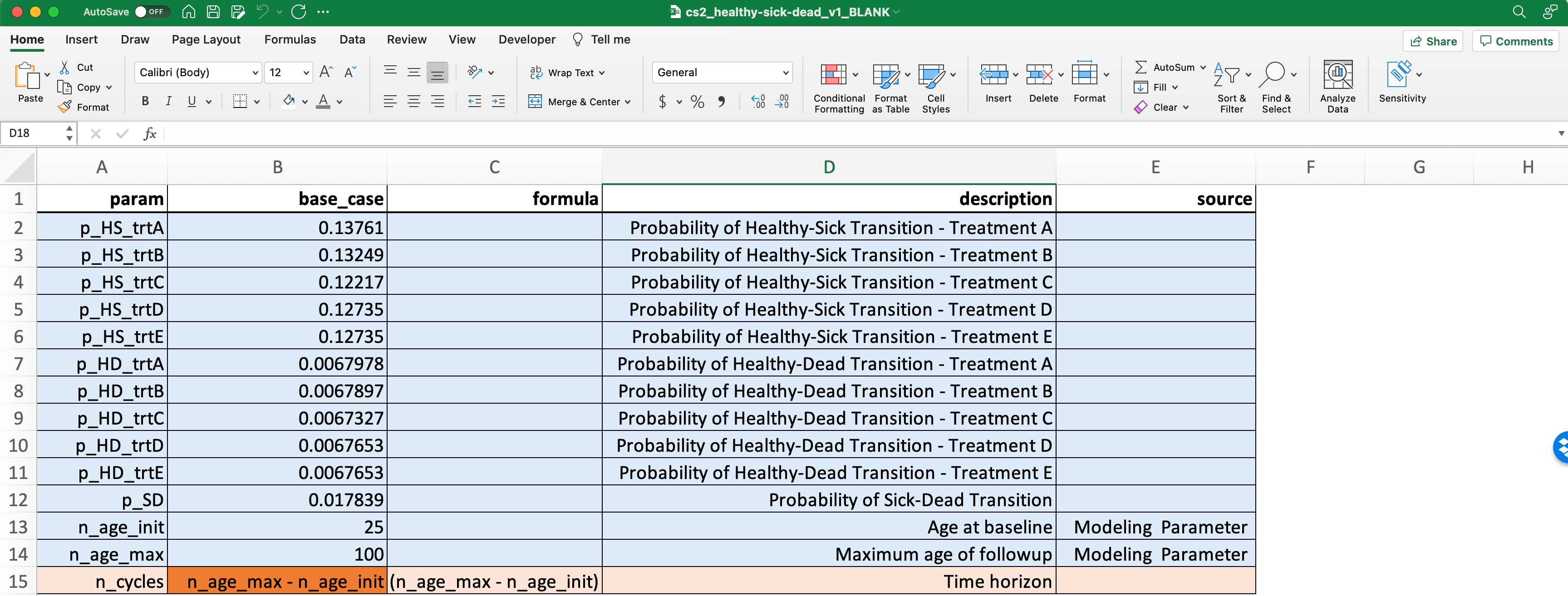
Notice that the rows are highlighted in two colors: blue and orange. The blue rows correspond to parameters that have fixed numeric values (e.g., p_HS_trtA is the probability of transitioning from healthy to sick under treatment A, and it has a value of 0.138).
By comparison, the orange rows highlight parameters that are functions of other parameters. The function that defines the parameter can be found in the formula column. In the table, the parameter n_cycles corresponds to the total number of Markov cycles our model will run. It is simply the difference between two other parameters: the starting age, and the maximum age of followup. In this example, the starting age (n_age_init) is 25 and the maximum followup (n_age_max) is 100. So we need to run 100 - 25 = 75 total cycles.
Why have we structured our table in this way? The simple answer is that we often want flexibility in how we model the decision problem–and it is good practice to structure your model such that any changes propagate through the model with a minimal amount of recoding/restructuring.
Suppose, for example, that instead of starting at age 25 we want to start at age 15. We could simply recode the n_age_init parameter to 15 and run the model. But because we have changed the starting age without changing the maximum age, we also change the total number of cycles we need to run!
If we had hard-coded 75 as the fixed value for n_cycles, we would end up running a Markov model that only runs until age 90 (i.e., 15+75). However, if we define n_cycles as a function of its input parameters n_age_max and n_age_init the spreadsheet will automatically update the value once we change one of the input parameters.
For these reasons it is best to structure your parameter tables by first thinking about which parameters are fixed values, and which parameters are simply functions of other parameters.
Step 1. Define Variable Names
For this case study the initial parameter table has already been constructed for you. However, to facilitate running the model we need to define each parameter for Excel.
The blog posting on useful Excel functions covers how to assign variable names in detail, and using several methods. Please take a few minutes to read through and watch the very short videos.
Once you are familiar with this process, complete Exercise 2.1 below.
Use variable names to assign values to each parameter in the Excel document.
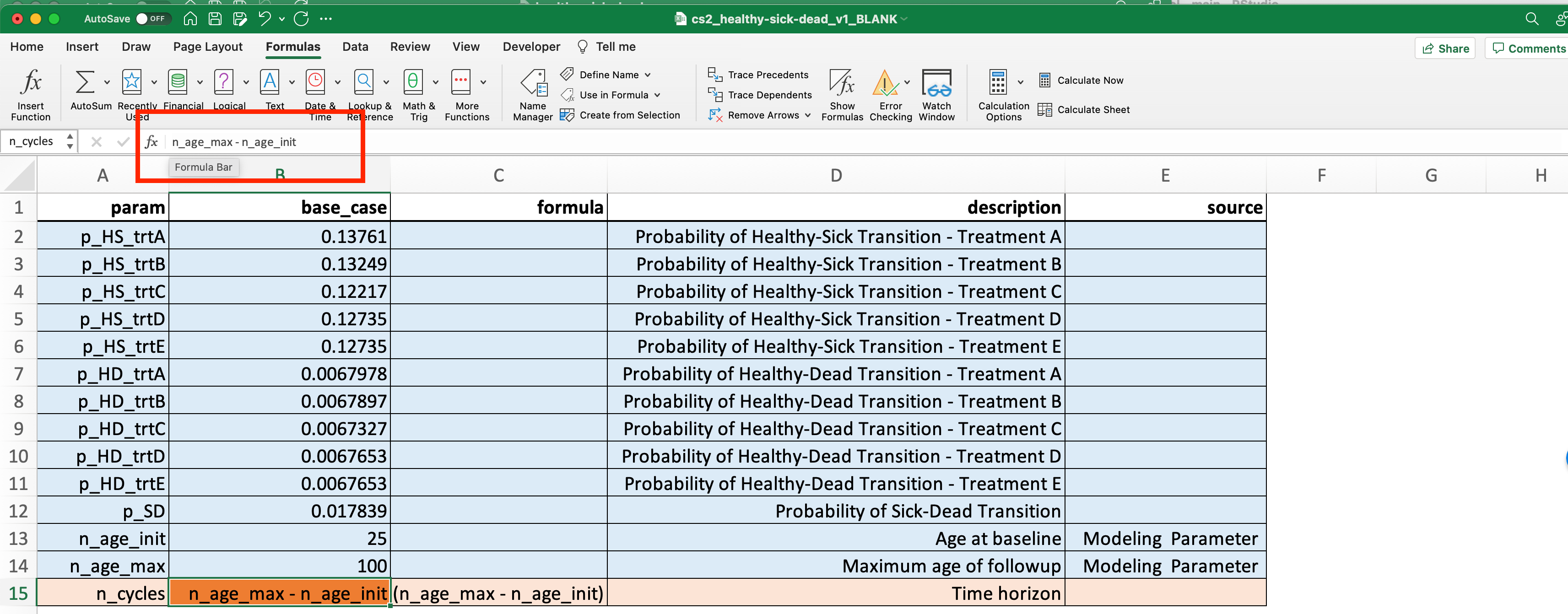
You may notice that the definition of n_cycles does not change once we define variables for all its inputs. To fix this, *in the base_case column, simply add an “=” sign to the formula in the formula input bar (see image below–the relevant cell where the formula is changed is B15 in the image). After doing so, the numeric value for this variable should appear.
Part 3: Define the Transition Probability Matrices
Define the Matrix Values
With the parameter names defined we can now define our transition probability matrices for each strategy. To do so, click on the tab for the first strategy (cs2_trtA). Notice that there is an empty transition probability matrix listed there:
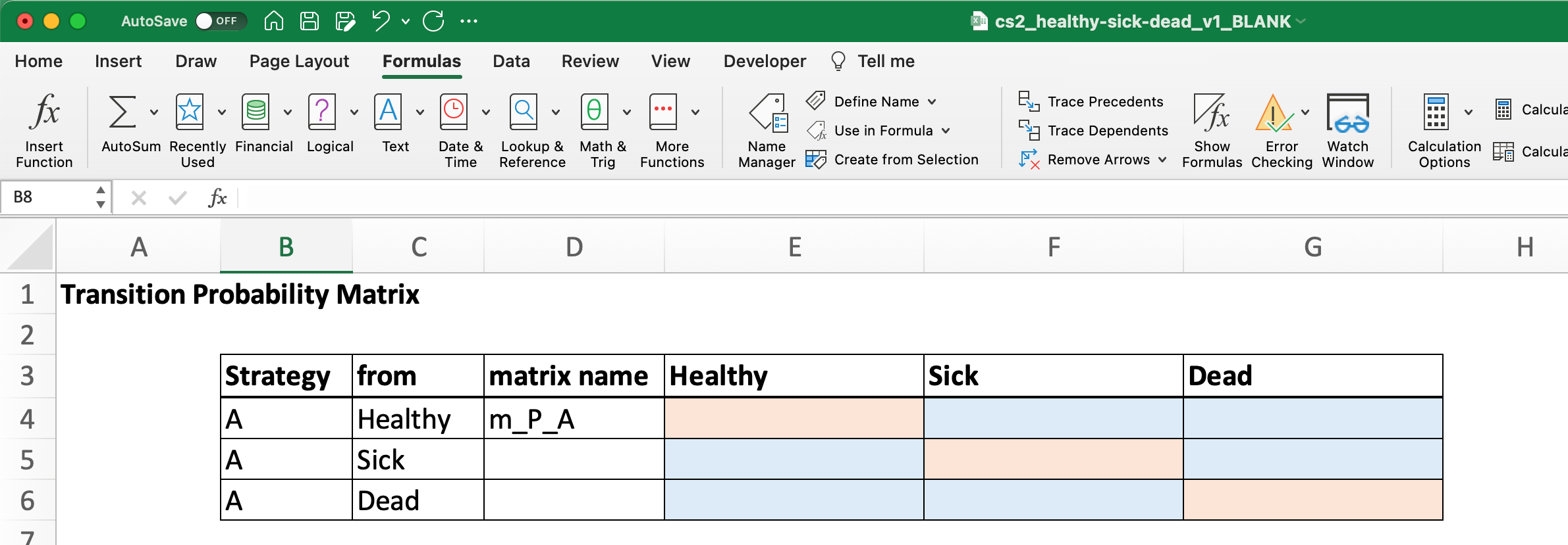
Recall from lecture that the diagonal elements of this matrix (i.e., those shaded in light red) should “balance out” the matrix so that the sum of all transition probabilities in a single row is equal to 1.0. That is why this row is also shaded in red; the value is obtained via a simple formula of other parameters.
Use the parameter names you just defined in Exercise 2.1 to fill out the transition probability matrix.
Don’t forget to include 0’s in cells where there is not an explicit transition probability!
Define the Matrix Name
Notice in cell D4 that we have defined a matrix name m_P_A. Our next step is to define a name for this matrix, much like we did for individual paramter values in Excercise 2.1.
The blog posting on useful Excel functions covers how to define names for matrices and other cell ranges (e.g., a column or row).
Define the name m_P_A for the transition probability matrix you just created.
To define the full matrix under a single name, you’ll need to select the full range of cells covered, and then assign a name. Also, you should only select the *cell values, not the row and column names.
Part 4: Construct the Markov Trace
With the transition probability matrix defined in terms of parameter names, and the matrix itself named, we can now construct a Markov trace using basic matrix multiplication.
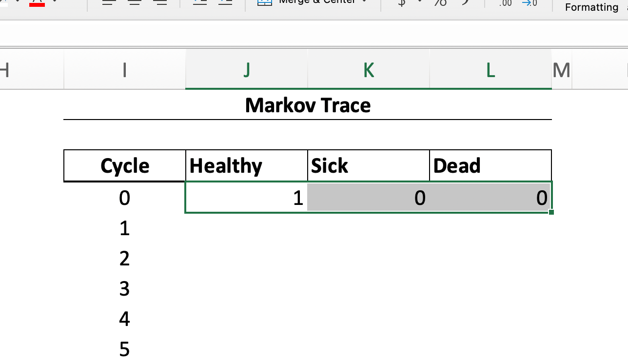
Figure Figure 3 provides a screenshot of an empty Markov trace that follows a hypothetical cohort who start out healthy (i.e., the values for Healthy, Sick, and Dead in cycle 0 are 1, 0 and 0, respectively).
100,000 in the Healthy cell.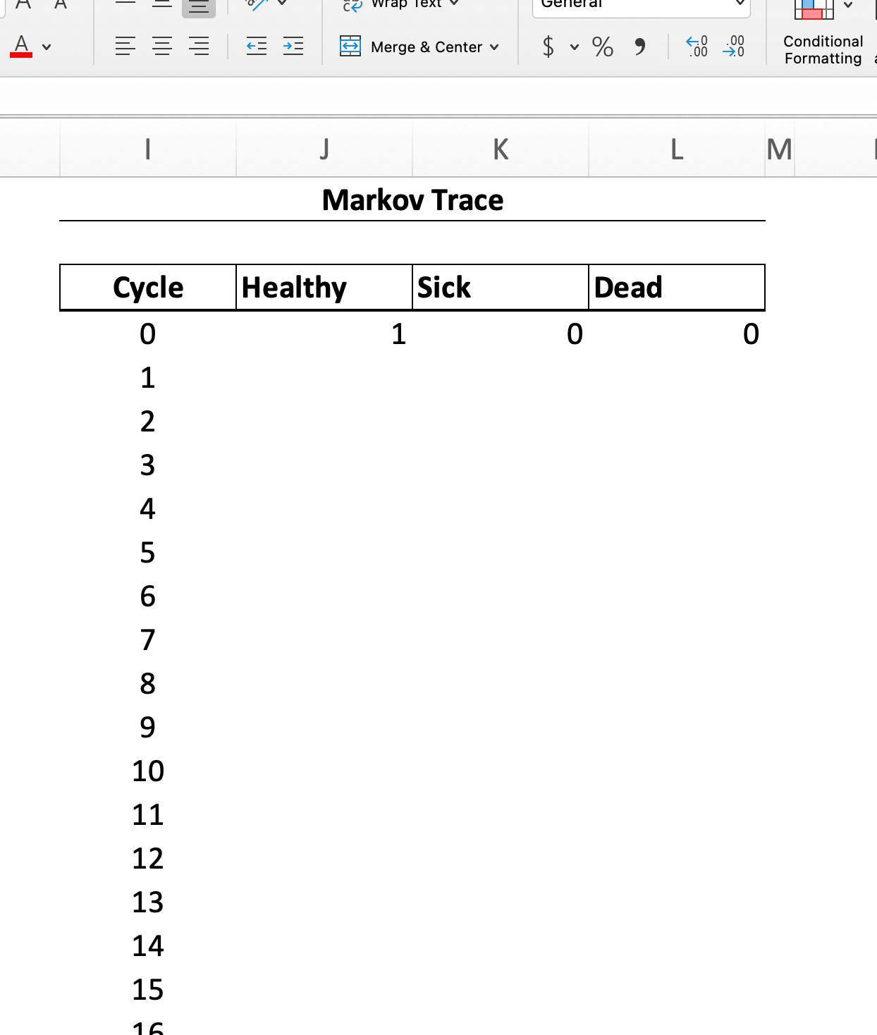
Calculating State Occupancy in a Given Cycle
The basic formula for state occupancy at any given time is
\[ s_t = s_{t-1}'m_P \] In Excel, \(m_P\) is the transition probability matrix you just defined. For cell cycle 1, \(s_{t-1}'\) corresponds to the highlighted cells in Figure 4 (i.e., the state occupancy of all states in cycle 0):
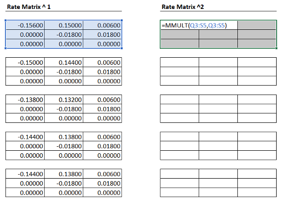
Finally, the matrix multiplication can be performed using the following command: MMULT(A,B), where A and B are the two things you want to multiply.
Use matrix multiplication to calculate state occupancy in cycle 1.
NOTE Depending on your Excel version, you may need to use a slightly different approach to ensure the MMULT() function executes.
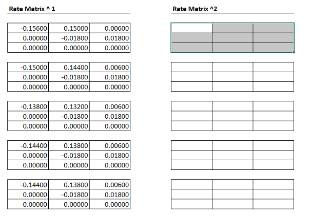
First, highlight the region you want to apply matrix multiplication to:
Next, enter the formula you want to execute:
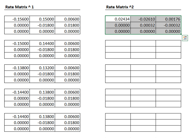
Finally, press control+shift+enter to get the formula to execute over the entire region of cells.
The blog post on useful Excel functions contains a video on how to construct a Markov trace.
NOTE Depending on your Excel version, you may need to use a slightly different approach to ensure the MMULT() function executes. First, try control+shift+enter to get the formula to execute. If that doesn’t work, flag Manny—he can help you work through this!
The matrix multiplication formula should be entered in the first state occupancy cell (i.e., “Healthy”) for the cycle.
Because everyone starts healthy in our model, it is straightforward to confirm we did the correct multiplication by looking at the transition probabilities in m_P_A.
Look at the transition probabilities in m_P_A. Does your Markov trace for cycle 1 reflect the correct transitions?
Part 5: Fill Out the Remaining Markov Traces
We now have the ingredients and processes needed to construct the full Markov trace for Strategy A, and for the other strategies. Each cycle is simply a replication of the matrix multiplication above.
Finish calculating the Markov trace for strategies A through E. Don’t forget to assign transition matrix names each time!